scipy.stats.uniform — SciPy v1.16.0 Manual (original) (raw)

scipy.stats.uniform = <scipy.stats._continuous_distns.uniform_gen object>[source]#

A uniform continuous random variable.

In the standard form, the distribution is uniform on [0, 1]. Using the parameters loc and scale, one obtains the uniform distribution on [loc, loc + scale].

As an instance of the rv_continuous class, uniform object inherits from it a collection of generic methods (see below for the full list), and completes them with details specific for this particular distribution.

Methods

Examples

import numpy as np from scipy.stats import uniform import matplotlib.pyplot as plt fig, ax = plt.subplots(1, 1)

Get the support:

lb, ub = uniform.support()

Calculate the first four moments:

mean, var, skew, kurt = uniform.stats(moments='mvsk')

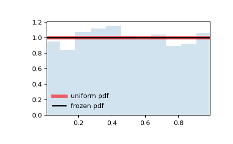
Display the probability density function (pdf):

x = np.linspace(uniform.ppf(0.01), ... uniform.ppf(0.99), 100) ax.plot(x, uniform.pdf(x), ... 'r-', lw=5, alpha=0.6, label='uniform pdf')

Alternatively, the distribution object can be called (as a function) to fix the shape, location and scale parameters. This returns a “frozen” RV object holding the given parameters fixed.

Freeze the distribution and display the frozen pdf:

rv = uniform() ax.plot(x, rv.pdf(x), 'k-', lw=2, label='frozen pdf')

Check accuracy of cdf and ppf:

vals = uniform.ppf([0.001, 0.5, 0.999]) np.allclose([0.001, 0.5, 0.999], uniform.cdf(vals)) True

Generate random numbers:

r = uniform.rvs(size=1000)

And compare the histogram:

ax.hist(r, density=True, bins='auto', histtype='stepfilled', alpha=0.2) ax.set_xlim([x[0], x[-1]]) ax.legend(loc='best', frameon=False) plt.show()