scipy.stats.vonmises — SciPy v1.16.2 Manual (original) (raw)

scipy.stats.vonmises = <scipy.stats._continuous_distns.vonmises_gen object>[source]#

A Von Mises continuous random variable.

As an instance of the rv_continuous class, vonmises object inherits from it a collection of generic methods (see below for the full list), and completes them with details specific for this particular distribution.

Methods

Notes

The probability density function for vonmises and vonmises_line is:

\[f(x, \kappa) = \frac{ \exp(\kappa \cos(x)) }{ 2 \pi I_0(\kappa) }\]

for \(-\pi \le x \le \pi\), \(\kappa \ge 0\). \(I_0\) is the modified Bessel function of order zero (scipy.special.i0).

vonmises is a circular distribution which does not restrict the distribution to a fixed interval. Currently, there is no circular distribution framework in SciPy. The cdf is implemented such thatcdf(x + 2*np.pi) == cdf(x) + 1.

vonmises_line is the same distribution, defined on \([-\pi, \pi]\)on the real line. This is a regular (i.e. non-circular) distribution.

Note about distribution parameters: vonmises and vonmises_line takekappa as a shape parameter (concentration) and loc as the location (circular mean). A scale parameter is accepted but does not have any effect.

Examples

Import the necessary modules.

import numpy as np import matplotlib.pyplot as plt from scipy.stats import vonmises

Define distribution parameters.

loc = 0.5 * np.pi # circular mean kappa = 1 # concentration

Compute the probability density at x=0 via the pdf method.

vonmises.pdf(0, loc=loc, kappa=kappa) 0.12570826359722018

Verify that the percentile function ppf inverts the cumulative distribution function cdf up to floating point accuracy.

x = 1 cdf_value = vonmises.cdf(x, loc=loc, kappa=kappa) ppf_value = vonmises.ppf(cdf_value, loc=loc, kappa=kappa) x, cdf_value, ppf_value (1, 0.31489339900904967, 1.0000000000000004)

Draw 1000 random variates by calling the rvs method.

sample_size = 1000 sample = vonmises(loc=loc, kappa=kappa).rvs(sample_size)

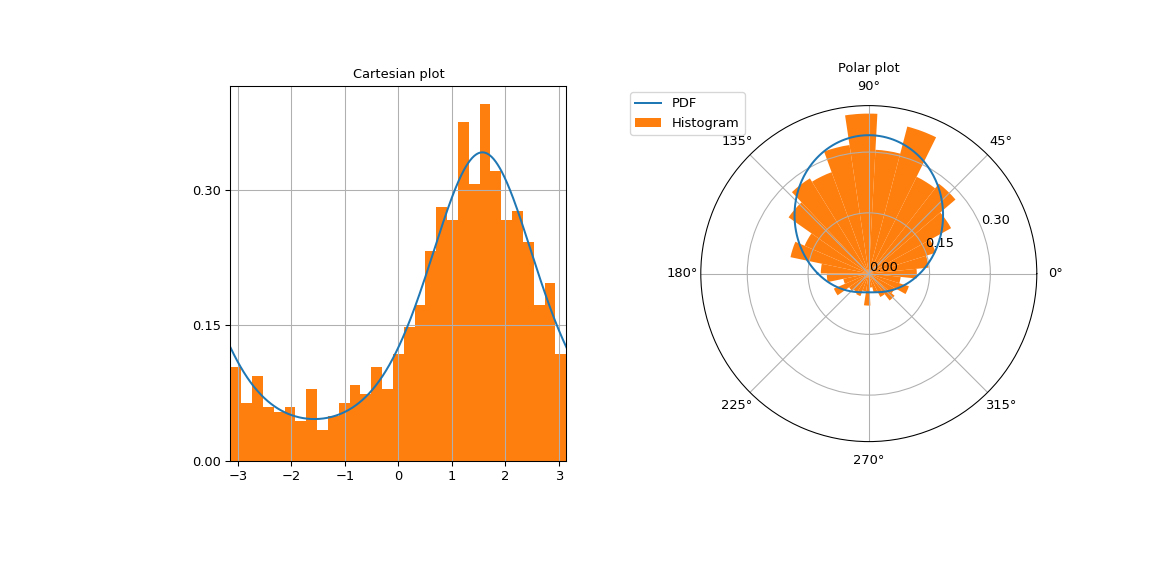
Plot the von Mises density on a Cartesian and polar grid to emphasize that it is a circular distribution.

fig = plt.figure(figsize=(12, 6)) left = plt.subplot(121) right = plt.subplot(122, projection='polar') x = np.linspace(-np.pi, np.pi, 500) vonmises_pdf = vonmises.pdf(x, loc=loc, kappa=kappa) ticks = [0, 0.15, 0.3]

The left image contains the Cartesian plot.

left.plot(x, vonmises_pdf) left.set_yticks(ticks) number_of_bins = int(np.sqrt(sample_size)) left.hist(sample, density=True, bins=number_of_bins) left.set_title("Cartesian plot") left.set_xlim(-np.pi, np.pi) left.grid(True)

The right image contains the polar plot.

right.plot(x, vonmises_pdf, label="PDF") right.set_yticks(ticks) right.hist(sample, density=True, bins=number_of_bins, ... label="Histogram") right.set_title("Polar plot") right.legend(bbox_to_anchor=(0.15, 1.06))