yeojohnson_normplot — SciPy v1.15.2 Manual (original) (raw)

scipy.stats.

scipy.stats.yeojohnson_normplot(x, la, lb, plot=None, N=80)[source]#

Compute parameters for a Yeo-Johnson normality plot, optionally show it.

A Yeo-Johnson normality plot shows graphically what the best transformation parameter is to use in yeojohnson to obtain a distribution that is close to normal.

Parameters:

xarray_like

Input array.

la, lbscalar

The lower and upper bounds for the lmbda values to pass toyeojohnson for Yeo-Johnson transformations. These are also the limits of the horizontal axis of the plot if that is generated.

plotobject, optional

If given, plots the quantiles and least squares fit.plot is an object that has to have methods “plot” and “text”. The matplotlib.pyplot module or a Matplotlib Axes object can be used, or a custom object with the same methods. Default is None, which means that no plot is created.

Nint, optional

Number of points on the horizontal axis (equally distributed from_la_ to lb).

Returns:

lmbdasndarray

The lmbda values for which a Yeo-Johnson transform was done.

ppccndarray

Probability Plot Correlation Coefficient, as obtained from probplotwhen fitting the Box-Cox transformed input x against a normal distribution.

Notes

Even if plot is given, the figure is not shown or saved byboxcox_normplot; plt.show() or plt.savefig('figname.png')should be used after calling probplot.

Added in version 1.2.0.

Examples

from scipy import stats import matplotlib.pyplot as plt

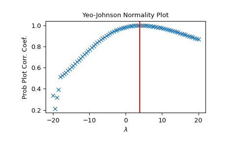
Generate some non-normally distributed data, and create a Yeo-Johnson plot:

x = stats.loggamma.rvs(5, size=500) + 5 fig = plt.figure() ax = fig.add_subplot(111) prob = stats.yeojohnson_normplot(x, -20, 20, plot=ax)

Determine and plot the optimal lmbda to transform x and plot it in the same plot:

_, maxlog = stats.yeojohnson(x) ax.axvline(maxlog, color='r')