Levenberg-Marquardt minimisation (original) (raw)

Next: Robust observations Up: The Vision Package Previous: Representing 3D Euclidean transformations Contents

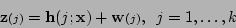
  #include <gandalf/vision/lev_marq.h>

The Levenberg-Marquardt algorithm [#!Marquardt:JSIAM63!#,#!Bjorck:96!#] is a general non-linear downhill minimisation algorithm for the case when derivatives of the objective function are known. It dynamically mixes Gauss-Newton and gradient-descent iterations. We shall develop the L-M algorithm for a simple case in our notation, which is derived from Kalman filtering theory [#!BarShalom:Fortmann:88!#]. The Gandalf implementation of Levenberg-Marquardt will then be presented. Let the unknown parameters be represented by the vector ${\bf x}$ , and let noisy measurements of ${\bf x}$ be made:

$\begin{displaymath} {\bf z}{\scriptstyle (j)}= {\bf h}(j;{\bf x}) + {\bf w}{\scriptstyle (j)},\;\;j=1,\ldots,k \end{displaymath}$	(5.7)

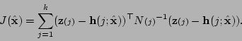
where ${\bf h}{\scriptstyle (j)}$ is a measurement function and ${\bf w}{\scriptstyle (j)}$ is zero-mean noise with covariance $N{\scriptstyle (j)}$ . Since we are describing an iterative minimization algorithm, we shall assume that we have already obtained an estimate $\hat{\bf x}^-$ of ${\bf x}$ . Then the maximum likelihood solution for a new estimate $\hat{\bf x}$ minimizes

$\begin{displaymath} J(\hat{\bf x}) = \sum_{j=1}^k({\bf z}{\scriptstyle (j)}-{\b... ...(j)}^{-1}({\bf z}{\scriptstyle (j)}-{\bf h}(j;\hat{\bf x})). \end{displaymath}$	(5.8)

We form a quadratic approximation to $J(.)$ around $\hat{\bf x}^-$ , and minimize this approximation to $J(.)$ to obtain a new estimate $\hat{\bf x}^+$ . In general we can write such a quadratic approximation as

$\begin{displaymath}J({\bf x}) \approx a - 2{\bf a}^{\top}({\bf x}-\hat{\bf x}^-) + ({\bf x}-\hat{\bf x}^-)^{\top}A ({\bf x}-\hat{\bf x}^-) \end{displaymath}$

for scalar $a$ , vectors ${\bf a}$ , ${\bf b}$ and matrices $A$ , $B$ . Note that here and in equation (5.8) the signs and factors of two are chosen WLOG to simplify the resulting expressions for the solution. Differentiating, we obtain

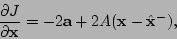
$\begin{displaymath} \frac{\partial J}{\partial {\bf x}} = - 2{\bf a}+ 2A({\bf x}-\hat{\bf x}^-), \;\;\;\; \end{displaymath}$

$\begin{displaymath} \frac{\partial^2 J}{\partial {\bf x}^2} = 2A, \;\;\;\; \end{displaymath}$

At the minimum point $\hat{\bf x}$ we have $\partial J/\partial {\bf x}={\bf0}$ which means that

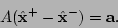$\begin{displaymath} A (\hat{\bf x}^+-\hat{\bf x}^-) = {\bf a}. \end{displaymath}$	(5.9)

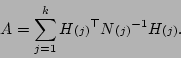
Thus we need to obtain ${\bf a}$ and $A$ to compute the update. We now consider the form of $J(.)$ in (5.8). Writing the Jacobian of ${\bf h}(j,{\bf x})$ as

$\begin{displaymath}H{\scriptstyle (j)}=\frac{\partial {\bf h}{\scriptstyle (j)}}{\partial {\bf x}}, \end{displaymath}$

we have

In the last formula for $\partial^2 J/\partial {\bf x}^2$ , the terms involving the second derivatives of ${\bf h}{\scriptstyle (j)}(.)$ have been omitted. This is done because these terms are generally much smaller and can in practice be omitted, as well as because the second derivatives are more difficult and complex to compute than the first derivatives.

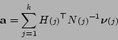
Now we solve the above equations for ${\bf a}$ and $A$ given the values of function ${\bf h}{\scriptstyle (j)}$ and the Jacobian $H{\scriptstyle (j)}$ evaluated at the previous estimate $\hat{\bf x}^-$ . We have immediately

$\begin{displaymath}A = \sum_{j=1}^kH{\scriptstyle (j)}^{\top}N{\scriptstyle (j)}^{-1}H{\scriptstyle (j)}. \end{displaymath}$

We now write the innovation vectors $\mbox{\boldmath$\nu$}{\scriptstyle (j)}$ as

$\begin{displaymath}\mbox{\boldmath$\nu$}{\scriptstyle (j)}= {\bf z}{\scriptstyle (j)}- {\bf h}(j;\hat{\bf x}^-) \end{displaymath}$

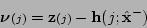
Then we have

$\begin{displaymath} {\bf a}= \sum_{j=1}^kH{\scriptstyle (j)}^{\top}N{\scriptstyle (j)}^{-1}\mbox{\boldmath$\nu$}{\scriptstyle (j)} \end{displaymath}$	(5.12)

Combining equations (5.9) and (5.12) we obtain the linear system

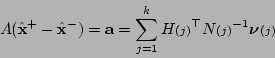$\begin{displaymath} A (\hat{\bf x}^+ - \hat{\bf x}^-) = {\bf a}= \sum_{j=1}^kH{... ...scriptstyle (j)}^{-1}\mbox{\boldmath$\nu$}{\scriptstyle (j)} \end{displaymath}$	(5.13)

to be solved for the adjustment $\hat{\bf x}^+ - \hat{\bf x}^-$ . The covariance of the state is

$\begin{displaymath}P = A^{-1}. \end{displaymath}$

The update (5.13) may be repeated, substituting the new $\hat{\bf x}^+$ as $\hat{\bf x}^-$ , and improving the estimate until convergence is achieved according to some criterion. Levenberg-Marquardt modifies this updating procedure by adding a value $\lambda$ to the diagonal elements of the linear system matrix before inverting it to obtain the update. $\lambda$ is reduced if the last iteration gave an improved estimate, i.e. if $J$ was reduced, and increased if $J$ increased, in which case the estimate of ${\bf x}$ is reset to the estimate before the last iteration. It is this that allows the algorithm to smoothly switch between Gauss-Newton (small $\lambda$ ) and gradient descent (large $\lambda$ ).

This version is a generalization of Levenberg-Marquardt as it is normally presented (e.g. [#!Press:etal:88!#]) in that we incorporate vector measurements ${\bf z}{\scriptstyle (j)}$ with covariances $N{\scriptstyle (j)}$ , rather than scalar measurements with variances. The full algorithm is as follows:

Start with a prior estimate $\hat{\bf x}^-$ of ${\bf x}$ . Initialize $\lambda$ to some starting value, e.g. 0.001.
Compute the updated estimate $\hat{\bf x}^+$ by solving the linear system (5.13) for the adjustment, having first added $\lambda$ to each diagonal element of . Note that the Lagrange multiplier diagonal block should remain at zero.
Compute the least-squares residuals and from (5.8).
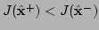1. If $J(\hat{\bf x}^+)<J(\hat{\bf x}^-)$ , reduce $\lambda$ by a specified factor (say 10), set $\hat{\bf x}^-$ to $\hat{\bf x}^+$ , and return to step 2.
2. Otherwise, the update failed to reduce the residual, so increase $\lambda$ by a factor (say 10), forget the updated $\hat{\bf x}^+$ and return to step 2. The algorithm continues until some pre-specified termination criterion has been met, such as a small change to the state vector, or a limit on the number of iterations.

If the measurements ${\bf z}{\scriptstyle (j)}$ are unbiased and normally distributed, the residual $J(\hat{\bf x}^+)$ is a $\chi^2$ random variable, and testing the value of $J$ against a $\chi^2$ distribution is a good way of checking that the measurement noise model is reasonable. The number of degrees of freedom (DOF) of the $\chi^2$ distribution can be determined as the total size of the measurement vectors, minus the size of the state. If the $SIZE(.)$ function returns the dimension of its vector argument, then the degrees of freedom may be computed as

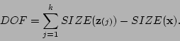$\begin{displaymath} DOF = \sum_{j=1}^kSIZE({\bf z}{\scriptstyle (j)}) - SIZE({\bf x}). \end{displaymath}$	(5.14)

Subsections

Next: Robust observations Up: The Vision Package Previous: Representing 3D Euclidean transformations Contents

2006-03-17