Image Segmentation (original) (raw)
Image segmentation models separate areas corresponding to different areas of interest in an image. These models work by assigning a label to each pixel. There are several types of segmentation: semantic segmentation, instance segmentation, and panoptic segmentation.
!pip install -q datasets transformers evaluate accelerate
We encourage you to log in to your Hugging Face account so you can upload and share your model with the community. When prompted, enter your token to log in:
from huggingface_hub import notebook_login
notebook_login()
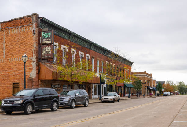
Semantic segmentation assigns a label or class to every single pixel in an image. Let’s take a look at a semantic segmentation model output. It will assign the same class to every instance of an object it comes across in an image, for example, all cats will be labeled as “cat” instead of “cat-1”, “cat-2”. We can use transformers’ image segmentation pipeline to quickly infer a semantic segmentation model. Let’s take a look at the example image.
from transformers import pipeline from PIL import Image import requests
url = "https://huggingface.co/datasets/huggingface/documentation-images/resolve/main/transformers/tasks/segmentation_input.jpg" image = Image.open(requests.get(url, stream=True).raw) image
semantic_segmentation = pipeline("image-segmentation", "nvidia/segformer-b1-finetuned-cityscapes-1024-1024") results = semantic_segmentation(image) results
The segmentation pipeline output includes a mask for every predicted class.
[{'score': None, 'label': 'road', 'mask': <PIL.Image.Image image mode=L size=612x415>}, {'score': None, 'label': 'sidewalk', 'mask': <PIL.Image.Image image mode=L size=612x415>}, {'score': None, 'label': 'building', 'mask': <PIL.Image.Image image mode=L size=612x415>}, {'score': None, 'label': 'wall', 'mask': <PIL.Image.Image image mode=L size=612x415>}, {'score': None, 'label': 'pole', 'mask': <PIL.Image.Image image mode=L size=612x415>}, {'score': None, 'label': 'traffic sign', 'mask': <PIL.Image.Image image mode=L size=612x415>}, {'score': None, 'label': 'vegetation', 'mask': <PIL.Image.Image image mode=L size=612x415>}, {'score': None, 'label': 'terrain', 'mask': <PIL.Image.Image image mode=L size=612x415>}, {'score': None, 'label': 'sky', 'mask': <PIL.Image.Image image mode=L size=612x415>}, {'score': None, 'label': 'car', 'mask': <PIL.Image.Image image mode=L size=612x415>}]
Taking a look at the mask for the car class, we can see every car is classified with the same mask.
In instance segmentation, the goal is not to classify every pixel, but to predict a mask for every instance of an object in a given image. It works very similar to object detection, where there is a bounding box for every instance, there’s a segmentation mask instead. We will use facebook/mask2former-swin-large-cityscapes-instance for this.
instance_segmentation = pipeline("image-segmentation", "facebook/mask2former-swin-large-cityscapes-instance") results = instance_segmentation(image) results
As you can see below, there are multiple cars classified, and there’s no classification for pixels other than pixels that belong to car and person instances.
[{'score': 0.999944, 'label': 'car', 'mask': <PIL.Image.Image image mode=L size=612x415>}, {'score': 0.999945, 'label': 'car', 'mask': <PIL.Image.Image image mode=L size=612x415>}, {'score': 0.999652, 'label': 'car', 'mask': <PIL.Image.Image image mode=L size=612x415>}, {'score': 0.903529, 'label': 'person', 'mask': <PIL.Image.Image image mode=L size=612x415>}]
Checking out one of the car masks below.
Panoptic segmentation combines semantic segmentation and instance segmentation, where every pixel is classified into a class and an instance of that class, and there are multiple masks for each instance of a class. We can use facebook/mask2former-swin-large-cityscapes-panoptic for this.
panoptic_segmentation = pipeline("image-segmentation", "facebook/mask2former-swin-large-cityscapes-panoptic") results = panoptic_segmentation(image) results
As you can see below, we have more classes. We will later illustrate to see that every pixel is classified into one of the classes.
[{'score': 0.999981, 'label': 'car', 'mask': <PIL.Image.Image image mode=L size=612x415>}, {'score': 0.999958, 'label': 'car', 'mask': <PIL.Image.Image image mode=L size=612x415>}, {'score': 0.99997, 'label': 'vegetation', 'mask': <PIL.Image.Image image mode=L size=612x415>}, {'score': 0.999575, 'label': 'pole', 'mask': <PIL.Image.Image image mode=L size=612x415>}, {'score': 0.999958, 'label': 'building', 'mask': <PIL.Image.Image image mode=L size=612x415>}, {'score': 0.999634, 'label': 'road', 'mask': <PIL.Image.Image image mode=L size=612x415>}, {'score': 0.996092, 'label': 'sidewalk', 'mask': <PIL.Image.Image image mode=L size=612x415>}, {'score': 0.999221, 'label': 'car', 'mask': <PIL.Image.Image image mode=L size=612x415>}, {'score': 0.99987, 'label': 'sky', 'mask': <PIL.Image.Image image mode=L size=612x415>}]
Let’s have a side by side comparison for all types of segmentation.
Seeing all types of segmentation, let’s have a deep dive on fine-tuning a model for semantic segmentation.
Common real-world applications of semantic segmentation include training self-driving cars to identify pedestrians and important traffic information, identifying cells and abnormalities in medical imagery, and monitoring environmental changes from satellite imagery.
To see all architectures and checkpoints compatible with this task, we recommend checking the task-page
Start by loading a smaller subset of the SceneParse150 dataset from the 🤗 Datasets library. This’ll give you a chance to experiment and make sure everything works before spending more time training on the full dataset.
from datasets import load_dataset
ds = load_dataset("scene_parse_150", split="train[:50]")
Split the dataset’s train split into a train and test set with the train_test_split method:
ds = ds.train_test_split(test_size=0.2) train_ds = ds["train"] test_ds = ds["test"]
train_ds[0] {'image': <PIL.JpegImagePlugin.JpegImageFile image mode=RGB size=512x683 at 0x7F9B0C201F90>, 'annotation': <PIL.PngImagePlugin.PngImageFile image mode=L size=512x683 at 0x7F9B0C201DD0>, 'scene_category': 368}
train_ds[0]["image"]
You’ll also want to create a dictionary that maps a label id to a label class which will be useful when you set up the model later. Download the mappings from the Hub and create the id2label and label2id dictionaries:
import json from pathlib import Path from huggingface_hub import hf_hub_download
repo_id = "huggingface/label-files" filename = "ade20k-id2label.json" id2label = json.loads(Path(hf_hub_download(repo_id, filename, repo_type="dataset")).read_text()) id2label = {int(k): v for k, v in id2label.items()} label2id = {v: k for k, v in id2label.items()} num_labels = len(id2label)
You could also create and use your own dataset if you prefer to train with the run_semantic_segmentation.py script instead of a notebook instance. The script requires:
As an example, take a look at this example dataset which was created with the steps shown above.
The next step is to load a SegFormer image processor to prepare the images and annotations for the model. Some datasets, like this one, use the zero-index as the background class. However, the background class isn’t actually included in the 150 classes, so you’ll need to set do_reduce_labels=True to subtract one from all the labels. The zero-index is replaced by 255 so it’s ignored by SegFormer’s loss function:
from transformers import AutoImageProcessor
checkpoint = "nvidia/mit-b0" image_processor = AutoImageProcessor.from_pretrained(checkpoint, do_reduce_labels=True)
Including a metric during training is often helpful for evaluating your model’s performance. You can quickly load an evaluation method with the 🤗 Evaluate library. For this task, load the mean Intersection over Union (IoU) metric (see the 🤗 Evaluate quick tour to learn more about how to load and compute a metric):
import evaluate
metric = evaluate.load("mean_iou")
Then create a function to compute the metrics. Your predictions need to be converted to logits first, and then reshaped to match the size of the labels before you can call compute:
Your compute_metrics function is ready to go now, and you’ll return to it when you setup your training.
Reload the dataset and load an image for inference.
from datasets import load_dataset
ds = load_dataset("scene_parse_150", split="train[:50]") ds = ds.train_test_split(test_size=0.2) test_ds = ds["test"] image = ds["test"][0]["image"] image
To visualize the results, load the dataset color palette as ade_palette() that maps each class to their RGB values.
def ade_palette(): return np.asarray([ [0, 0, 0], [120, 120, 120], [180, 120, 120], [6, 230, 230], [80, 50, 50], [4, 200, 3], [120, 120, 80], [140, 140, 140], [204, 5, 255], [230, 230, 230], [4, 250, 7], [224, 5, 255], [235, 255, 7], [150, 5, 61], [120, 120, 70], [8, 255, 51], [255, 6, 82], [143, 255, 140], [204, 255, 4], [255, 51, 7], [204, 70, 3], [0, 102, 200], [61, 230, 250], [255, 6, 51], [11, 102, 255], [255, 7, 71], [255, 9, 224], [9, 7, 230], [220, 220, 220], [255, 9, 92], [112, 9, 255], [8, 255, 214], [7, 255, 224], [255, 184, 6], [10, 255, 71], [255, 41, 10], [7, 255, 255], [224, 255, 8], [102, 8, 255], [255, 61, 6], [255, 194, 7], [255, 122, 8], [0, 255, 20], [255, 8, 41], [255, 5, 153], [6, 51, 255], [235, 12, 255], [160, 150, 20], [0, 163, 255], [140, 140, 140], [250, 10, 15], [20, 255, 0], [31, 255, 0], [255, 31, 0], [255, 224, 0], [153, 255, 0], [0, 0, 255], [255, 71, 0], [0, 235, 255], [0, 173, 255], [31, 0, 255], [11, 200, 200], [255, 82, 0], [0, 255, 245], [0, 61, 255], [0, 255, 112], [0, 255, 133], [255, 0, 0], [255, 163, 0], [255, 102, 0], [194, 255, 0], [0, 143, 255], [51, 255, 0], [0, 82, 255], [0, 255, 41], [0, 255, 173], [10, 0, 255], [173, 255, 0], [0, 255, 153], [255, 92, 0], [255, 0, 255], [255, 0, 245], [255, 0, 102], [255, 173, 0], [255, 0, 20], [255, 184, 184], [0, 31, 255], [0, 255, 61], [0, 71, 255], [255, 0, 204], [0, 255, 194], [0, 255, 82], [0, 10, 255], [0, 112, 255], [51, 0, 255], [0, 194, 255], [0, 122, 255], [0, 255, 163], [255, 153, 0], [0, 255, 10], [255, 112, 0], [143, 255, 0], [82, 0, 255], [163, 255, 0], [255, 235, 0], [8, 184, 170], [133, 0, 255], [0, 255, 92], [184, 0, 255], [255, 0, 31], [0, 184, 255], [0, 214, 255], [255, 0, 112], [92, 255, 0], [0, 224, 255], [112, 224, 255], [70, 184, 160], [163, 0, 255], [153, 0, 255], [71, 255, 0], [255, 0, 163], [255, 204, 0], [255, 0, 143], [0, 255, 235], [133, 255, 0], [255, 0, 235], [245, 0, 255], [255, 0, 122], [255, 245, 0], [10, 190, 212], [214, 255, 0], [0, 204, 255], [20, 0, 255], [255, 255, 0], [0, 153, 255], [0, 41, 255], [0, 255, 204], [41, 0, 255], [41, 255, 0], [173, 0, 255], [0, 245, 255], [71, 0, 255], [122, 0, 255], [0, 255, 184], [0, 92, 255], [184, 255, 0], [0, 133, 255], [255, 214, 0], [25, 194, 194], [102, 255, 0], [92, 0, 255], ])
import matplotlib.pyplot as plt import numpy as np
color_seg = np.zeros((pred_seg.shape[0], pred_seg.shape[1], 3), dtype=np.uint8) palette = np.array(ade_palette()) for label, color in enumerate(palette): ... color_seg[pred_seg == label, :] = color color_seg = color_seg[..., ::-1]
img = np.array(image) * 0.5 + color_seg * 0.5
img = img.astype(np.uint8)
plt.figure(figsize=(15, 10)) plt.imshow(img) plt.show()