Classify Motor Faults Using Deep Learning - MATLAB & Simulink (original) (raw)

Main Content

This example shows how to train a deep learning model to classify faults in a permanent magnet synchronous motor (PMSM) using simulated data across various revolutions per minute (RPM). You use Simscape Electrical™ to create the model for a fault scenario, then use Deep Learning Toolbox™ to train a neural network to classify the fault data.

Detecting and classifying faults in electric motors is essential for maintaining system reliability and safety. If you do not address faults promptly, they can decrease performance, increase operational costs, and even cause catastrophic failures, such as the loss of control over motor speed. By accurately identifying faults, you can schedule maintenance proactively, which minimizes downtime and extends the life of a motor. Advanced fault detection techniques, such as those using deep learning, provide precise and efficient solutions for real-time fault classification.

Identify Types of PMSM Faults

These types of internal electromagnetic faults occur in PMSMs:

Open-circuit fault — This fault occurs when one of the electrical terminals disconnects, leading to reduced torque and possible overheating.
Coil-grounded fault — This fault occurs when a winding shorts to ground, potentially causing unbalanced currents and increased losses.
Isolated turns in a coil — This fault occurs when one of the turns in the coil short-circuits, leading to localized heating and reduced efficiency.
Rotor demagnetization — This fault occurs when the field strength of the rotor reduces, leading to lower torque and efficiency.

Motors can also experience mechanical faults and sensor faults. This example focuses only on the internal electromagnetic faults.

Mitigate Fault Effects

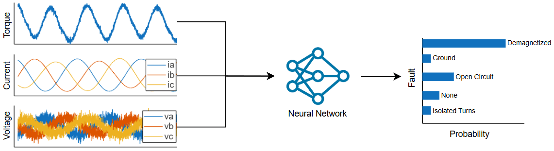
You can design control systems to detect faults and mitigate fault effects. This example focuses on the detection and classification of faults. In this example, you train a 1-D convolutional neural network (CNN) with these inputs:

Torque
A-phase, B-phase, and C-phase currents
A-phase, B-phase, and C-phase voltages

The CNN returns the predicted fault of the simulated data as output. You then validate the trained model against real-world measurements and can deploy the validated model to classify faults in real time.

Generate Data

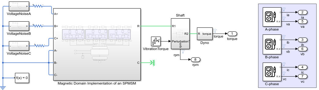
The PMSM model in this example is a three-phase, inrunner, radial-flux surface permanent magnet synchronous motor (SPMSM) with ten rotor poles and nine stator winding slots. This model is adapted from the model in the Faulted PMSM (Simscape Electrical) example.

A PMSM model typically represents each winding as a single entity with associated inductance, induced back electromotive force (EMF), and mutual inductive coupling to adjacent windings. However, this simplified model breaks down when a winding fault occurs. To accurately capture the dynamics of a faulted motor, you must model the motor at the winding slot level in the magnetic domain. This more detailed model accurately represents the effects of faults on the magnetic circuit of the motor.

To effectively train a deep learning model for fault classification, it is crucial to generate fault data across a range of RPM. Generating data from a range of RPM ensures that you capture the performance of the motor under various operational conditions. PMSMs can function as both motors, which converts electrical power into mechanical power, and generators, which convert mechanical power into electrical power.

In this example, data collection focuses on a PMSM functioning as a generator. When a PMSM acts as a generator, the shaft spins at a constant speed, allowing the back-EMF to produce electrical current in resistors connected in a wye configuration. The motor acts as a load that supplies power to the resistors, causing the motor to operate as an open-loop generator like a dynamo. In this example, the training data collected using the fault classification algorithm is only a PMSM acting as a generator. To enable fault classification for a PMSM acting as a motor, you must modify the model to collect training data specifically for that mode.

Use the FaultedPMSM Simulink® model to generate the data.

motorModel = "FaultedPMSM";

Specify to generate data for four types of faults (demagnetized, ground, isolated turns, and open-circuit) and data for no faults:

faults = ["Demagnetized" "Ground" "IsolatedTurns" "None" "OpenCircuit"]; dataInfo.faults = faults;

Specify to generate data at intervals of 25 RPM between -250 and -50 RPM and between 50 and 250 RPM.

rpmStep = 25;

speedValuesRPMNegative = -250:rpmStep:-50; speedValuesRPMPositive = 50:rpmStep:250;

speedValuesRPM = [speedValuesRPMNegative speedValuesRPMPositive];

During simulation, there is an initial period before the motor settles into its operating point. To ensure that the training data is reflective of the true model performance, specify a warm-up period of 0.25 seconds before saving the data. The warm-up period removes the initial dynamic transient. The length of the warm-up period is dependent on your data. You can choose the warm-up period by inspecting your data.

Generate the data using the helper function generateAndSavePMSMFaultDataForSpeed. To access this function, open the example live script. Generating the data can take a few minutes. If you have already generated the data, then set generateData to false.

generateData = true;

if generateData mkdir("FaultData") for idxCase = 1:numel(speedValuesRPM) disp("Generate data for " + speedValuesRPM(idxCase) + " RPM"); generateAndSavePMSMFaultDataForSpeed(motorModel,speedValuesRPM(idxCase),faults,warmupPeriod) end end

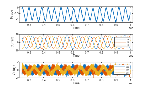
Plot Generated Data

Plot an example of the generated data.

firstRPMData = load("FaultData\FaultedPMSMResults" + speedValuesRPM(1) + "RPM"); exampleGeneratedData = firstRPMData.Demagnetized_ResultsInSIUnits;

tiledlayout(3,1) nexttile plot(exampleGeneratedData,"torque") ylabel("Torque")

nexttile plot(exampleGeneratedData,["ia","ib","ic"]) ylabel("Current") legend

nexttile plot(exampleGeneratedData,["va","vb","vc"]) ylabel("Voltage") legend

Prepare Data for Training Deep Neural Network

Prepare the data for training a deep learning model. Create a training set that contains data for positive and negative RPM. Hold some of the data to use as unseen test data. The held data shows how well the deep learning model performs for simulations with an RPM that it was not trained on.

trainRPMNegative = speedValuesRPMNegative(1:2:end); trainRPMPositive = speedValuesRPMPositive(1:2:end);

trainRPM = [trainRPMNegative trainRPMPositive]

trainRPM = 1×10

-250 -200 -150 -100 -50 50 100 150 200 250

testRPM = setdiff(speedValuesRPM,trainRPM)

testRPM = 1×8

-225 -175 -125 -75 75 125 175 225

In frame-based processing, the software processes data in frames, also known as chunks. Each frame of data contains samples of consecutive times stacked together. Each feature is represented by a column of the input signal. Splitting the data into frames can help speed up the training of the neural network. Use the helper function prepareFaultData to split the data into frames. Specify an overlap to ensure that the training data captures all of the simulation behavior. The frame size and amount of the overlap are tunable hyperparameters that depend on your data. The frame size during inference must be the same size as the size you use during training.

frameSize = 500; dataInfo.frameSize = frameSize; save("dataInfo","dataInfo")

overlap = 100; [XData,YData] = prepareFaultData(trainRPM,frameSize,overlap);

Split Data into Training and Validation Sets

Use the helper function splitData to split the training data into a training set and a validation set. The neural network does not use the validation data to train. Instead, the validation data allows you to see how well the neural network performs during training.

trainingPercentage = 0.8; [XTrain,YTrain,XVal,YVal] = splitData(XData,YData,trainingPercentage);

Build Deep Neural Network

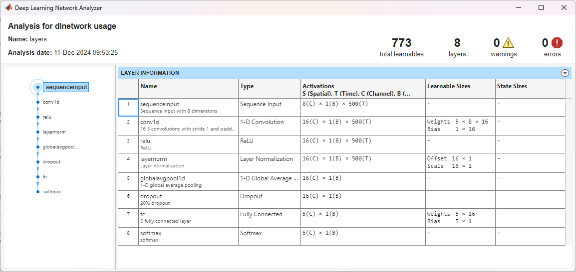
Create a 1-D CNN suitable for sequence-to-one classification tasks. In this example, the network must take as input eight features and must classify the data into one of five classes.

Use a sequence input layer with an input size equal to the number of input signals and the minimum length equal to the frame size. In this example, the network takes as input the torque, three current values, three voltage values, and the RPM.
Use a convolution 1-D layer followed by a ReLU layer, a layer normalization layer, and a 1-D global average pooling layer.
Add a dropout layer to improve the generalization of the network.
Add a fully connected layer with a number of outputs equal to the number of classes.
As this is a classification task, use a softmax layer as the final layer.

numFeatures = 8; numClasses = 5;

layers = [ ... sequenceInputLayer(numFeatures,MinLength=frameSize,Normalization="zscore") convolution1dLayer(5,16,Padding="same") reluLayer layerNormalizationLayer
globalAveragePooling1dLayer dropoutLayer(0.2) fullyConnectedLayer(numClasses) softmaxLayer];

Use the analyzeNetwork function to see the size of the model. In this example, the network is very small with less then 1000 learnable parameters.

info = analyzeNetwork(layers);

Determine the memory footprint of the model in kilobytes (KB). The software stores the learnables as four bytes, so you can easily estimate the size of the network.

networkSizeInKB = info.TotalLearnables*(4/(1024^2))*1000

Train Model

Specify the training options. To explore different training option configurations by running experiments, you can use the Experiment Manager app.

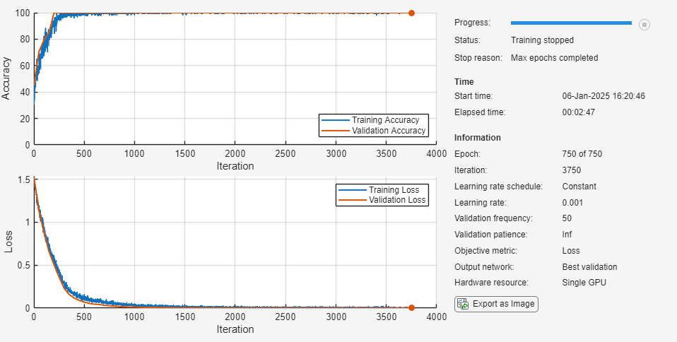
options = trainingOptions("adam", ... MaxEpochs=750, ... Verbose=0, ... Shuffle="every-epoch", ... Plots="training-progress", ... ValidationData={XVal,YVal}, ... Metrics = "accuracy");

Train the neural network using the trainnet function. For classification tasks, use cross-entropy loss. By default, the trainnet function uses a GPU if one is available. Training on a GPU requires a Parallel Computing Toolbox™ license and a supported GPU device. For information on supported devices, see GPU Computing Requirements (Parallel Computing Toolbox). If a GPU is not available, the trainnet function uses the CPU. To select the execution environment manually, use the ExecutionEnvironment training option.

net = trainnet(XTrain,YTrain,layers,"crossentropy",options);

Save the trained model.

save("trainedFaultClassifierModel.mat","net")

Test Model

Test the trained network on the test data taken at unseen RPM values. The network achieves a high accuracy even though it was not specifically trained on data at these RPM values.

[XTest,YTest] = prepareFaultData(testRPM,frameSize,overlap); testnet(net,XTest,YTest,"accuracy")

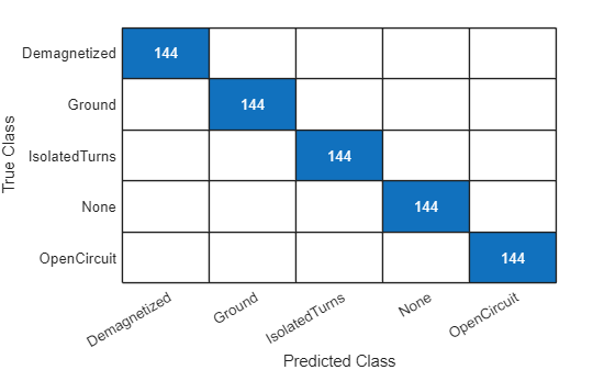
Generate a confusion chart to see the network performance across each fault.

YPredTest = minibatchpredict(net,XTest); YPredTest = onehotdecode(YPredTest,faults,2);

figure confusionchart(YTest,YPredTest);

Test Model in Simulink

Test the performance of the trained network in Simulink® using the FaultClassifier_CNN model. This model uses the FaultedPMSM model to simulate the fault data and then classifies it using the trained neural network. The model incorporates the trained network as a series of layer blocks that correspond to the layers in the network. You can convert a neural network to Simulink layer blocks using the exportNetworkToSimulink function. To pass the network frame sizes at the same size as the frames used in training, the model uses a Buffer (DSP System Toolbox) block to create the frames.

classifierModel = "FaultClassifier_CNN"; open_system(classifierModel) load_system(motorModel); FaultedPMSMParameters;

Specify the fault and set the trigger time between 0 and 4. Specify any RPM. The neural network has been trained on values between -250 and 250 RPM, but you can also see how it performs for RPM values outside of that range.

motorRPM = 150;

Simulate the specified fault and use the neural network to classify it.

FaultedPMSMSetFault(classifierModel,fault,triggerTime);

Fault scenario: IsolatedTurns

faultSignal = getFaultSignal(fault,faults,triggerTime); simOut = sim(classifierModel);

Log the true and predicted fault values.

logsout_PMSMFaultClassifier = simOut.logsout_PMSMFaultClassifier; predictedFault = get(logsout_PMSMFaultClassifier,"predicted_fault").Values; trueFault = get(logsout_PMSMFaultClassifier,"true_fault").Values;

[predictedFault, trueFault] = synchronize(predictedFault,trueFault,"Intersection");

Evaluate the accuracy of the neural network across the full signal. When computing the accuracy, exclude the first five predictions, which correspond to the warm-up period.

warmupFramesToExclude = 5; predValues = predictedFault.Data(warmupFramesToExclude+1:end); trueValues = trueFault.Data(warmupFramesToExclude+1:end); simAccuracy = 100*sum(predValues==trueValues)/numel(predValues)

Compute the time it takes for the neural network to detect the fault after it triggers. To calculate the sample time of the network, multiply the value of frameSize by solverSampleTime. In this example, the sample time is 0.05 seconds. During this simulation, it takes two time steps to identify the fault.

postTriggerResponse = predictedFault.Data(predictedFault.Time>=triggerTime,:) == trueFault.Data(trueFault.Time>=triggerTime,:); stepsForFaultDetection = find(postTriggerResponse == 1, 1);

timeForDetection = stepsForFaultDetection * seconds((predictedFault.Time(2)-predictedFault.Time(1)))

timeForDetection = duration 0.1 sec