Use Experiment Manager to Train Generative Adversarial Networks (GANs) - MATLAB & Simulink (original) (raw)

This example shows how to create a custom training experiment to train a generative adversarial network (GAN) that generates images of flowers. For a custom training experiment, you explicitly define the training procedure used by Experiment Manager. In this example, you implement a custom training loop to train a GAN, a type of deep learning network that can generate data with similar characteristics as the input real data. A GAN consists of two networks that train together:

Generator — Given a vector of random values (latent inputs) as input, this network generates data with the same structure as the training data.
Discriminator — Given batches of data containing observations from both the training data, and generated data from the generator, this network attempts to classify the observations as "real" or "generated."

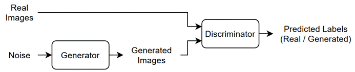
To train a GAN, train both networks simultaneously to maximize the performance of both networks:

Train the generator to generate data that "fools" the discriminator. To optimize the performance of the generator, maximize the loss of the discriminator when given generated data. In other words, the objective of the generator is to generate data that the discriminator classifies as "real."
Train the discriminator to distinguish between real and generated data. To optimize the performance of the discriminator, minimize the loss of the discriminator when given batches of both real and generated data. In other words, the objective of the discriminator is to not be "fooled" by the generator.

Ideally, these strategies result in a generator that generates convincingly realistic data and a discriminator that has learned strong feature representations that are characteristic of the training data. For more information, see Train Generative Adversarial Network (GAN).

Open Experiment

First, open the example. Experiment Manager loads a project with a preconfigured experiment that you can inspect and run. To open the experiment, in the Experiment Browser pane, double-click ImageGenerationExperiment.

Custom training experiments consist of a description, a table of hyperparameters, and a training function. For more information, see Train Network Using Custom Training Loop and Display Visualization.

The Description field contains a textual description of the experiment. For this example, the description is:

Train a generative adversarial network (GAN) to generate images of flowers. Use hyperparameters to specify:

the probability of the dropout layer in the discriminator network
the fraction of real labels to flip while training the discriminator network

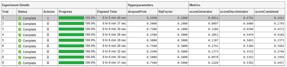
The Hyperparameters section specifies the strategy and hyperparameter values to use for the experiment. When you run the experiment, Experiment Manager trains the network using every combination of hyperparameter values specified in the hyperparameter table. This example uses two hyperparameters:

dropoutProb sets the probability of the dropout layer in the discriminator network. By default, the values for this hyperparameter are specified as [0.25 0.5 0.75].
flipFactor sets the fraction of real labels to flip when you train the discriminator network. The experiment uses this hyperparameter to add noise to the real data and better balance the learning of the discriminator and the generator. Otherwise, if the discriminator learns to discriminate between real and generated images too quickly, then the generator can fail to train. The values for this hyperparameter are specified as [0.1 0.3 0.5].

The Training Function section specifies a function that defines the training data, network architecture, training options, and training procedure used by the experiment. To open this function in MATLAB® Editor, click Edit. The code for the function also appears in Training Function. The input to the training function is a structure with fields from the hyperparameter table and an experiments.Monitor object that you can use to track the progress of the training, record values of the metrics used by the training, and produce training plots. The function returns a structure that contains the trained generator network, the trained discriminator network, and the execution environment used for training. Experiment Manager saves this output so you can export it to the MATLAB workspace when the training is complete. The training function has these sections:

Initialize Output sets the initial value of the networks to empty arrays to indicate that the training has not started. The experiment sets the execution environment to "auto", so it trains the networks on a GPU if one is available. Using a GPU requires Parallel Computing Toolbox™ and a supported GPU device. For more information, see GPU Computing Requirements (Parallel Computing Toolbox).

output.generator = []; output.discriminator = []; output.executionEnvironment = "auto";

Load Training Data defines the training data for the experiment as an imageDatastore object. The experiment uses the Flowers data set, which contains 3670 images of flowers and is about 218 MB. For more information on this data set, see Image Data Sets.

monitor.Status = "Loading Data";

url = "http://download.tensorflow.org/example_images/flower_photos.tgz"; downloadFolder = tempdir; filename = fullfile(downloadFolder,"flower_dataset.tgz");

imageFolder = fullfile(downloadFolder,"flower_photos"); if ~exist(imageFolder,"dir") websave(filename,url); untar(filename,downloadFolder) end

datasetFolder = fullfile(imageFolder); imdsTrain = imageDatastore(datasetFolder, ... IncludeSubfolders=true);

augmenter = imageDataAugmenter(RandXReflection=true); augimdsTrain = augmentedImageDatastore([64 64],imdsTrain, ... DataAugmentation=augmenter);

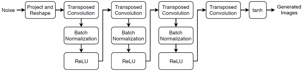
Define Generator Network defines the architecture for the generator network as a layer graph that generates images from 1-by-1-by-100 arrays of random values. To train the network with a custom training loop and enable automatic differentiation, the training function converts the layer graph to a dlnetwork object. The generator network has this architecture:

monitor.Status = "Creating Generator";

filterSize = 5; numFilters = 64; numLatentInputs = 100; projectionSize = [4 4 512];

layersGenerator = [ featureInputLayer(numLatentInputs) projectAndReshapeLayer(projectionSize,Name="proj") transposedConv2dLayer(filterSize,4numFilters) batchNormalizationLayer reluLayer transposedConv2dLayer(filterSize,2numFilters,Stride=2,Cropping="same") batchNormalizationLayer reluLayer transposedConv2dLayer(filterSize,numFilters,Stride=2,Cropping="same") batchNormalizationLayer reluLayer transposedConv2dLayer(filterSize,3,Stride=2,Cropping="same") tanhLayer];

lgraphGenerator = layerGraph(layersGenerator); output.generator = dlnetwork(lgraphGenerator);

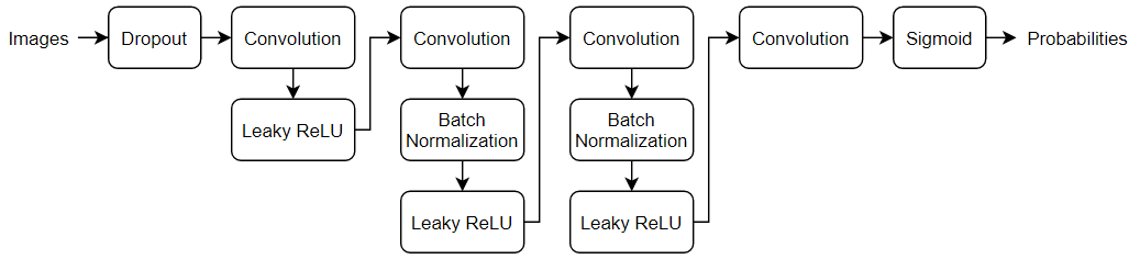
Define Discriminator Network defines the architecture for the discriminator network as a layer graph that classifies real and generated 64-by-64-by-3 images. The dropout layer uses the dropout probability defined in the hyperparameter table. To train the network with a custom training loop and enable automatic differentiation, the training function converts the layer graph to a dlnetwork object. The discriminator network has this architecture:

monitor.Status = "Creating Discriminator";

filterSize = 5; numFilters = 64; inputSize = [64 64 3]; dropoutProb = params.dropoutProb; scale = 0.2;

layersDiscriminator = [ imageInputLayer(inputSize,Normalization="none") dropoutLayer(dropoutProb) convolution2dLayer(filterSize,numFilters,Stride=2,Padding="same") leakyReluLayer(scale) convolution2dLayer(filterSize,2numFilters,Stride=2,Padding="same") batchNormalizationLayer leakyReluLayer(scale) convolution2dLayer(filterSize,4numFilters,Stride=2,Padding="same") batchNormalizationLayer leakyReluLayer(scale) convolution2dLayer(filterSize,8*numFilters,Stride=2,Padding="same") batchNormalizationLayer leakyReluLayer(scale) convolution2dLayer(4,1) sigmoidLayer];

lgraphDiscriminator = layerGraph(layersDiscriminator); output.discriminator = dlnetwork(lgraphDiscriminator);

Specify Training Options defines the training options used by the experiment. In this example, Experiment Manager trains the networks with a mini-batch size of 128 for 50 epochs using an initial learning rate of 0.0002, a gradient decay factor of 0.5, and a squared gradient decay factor of 0.999.

numEpochs = 50; miniBatchSize = 128; learnRate = 0.0002; gradientDecayFactor = 0.5; squaredGradientDecayFactor = 0.999; trailingAvgG = []; trailingAvgSqG = []; trailingAvgD = []; trailingAvgSqD = []; flipFactor = params.flipFactor;

Train Model defines the custom training loop used by the experiment. The custom training loop uses minibatchqueue to process and manage the mini-batches of images. For each mini-batch, the minibatchqueue object rescales the images in the range [-1,1], discards any partial mini-batches with fewer than 128 observations, and formats the image data with the dimension labels "SSCB" (spatial, spatial, channel, batch). By default, the minibatchqueue object converts the data to dlarray objects with underlying type single. For each epoch, the custom training loop shuffles the datastore and loops over mini-batches of data. If you train on a GPU, the data is converted to gpuArray (Parallel Computing Toolbox) objects. Then, the training function evaluates the model gradients and updates the discriminator and generator network parameters. After each iteration of the custom training loop, the training function saves the trained networks and updates the training progress.

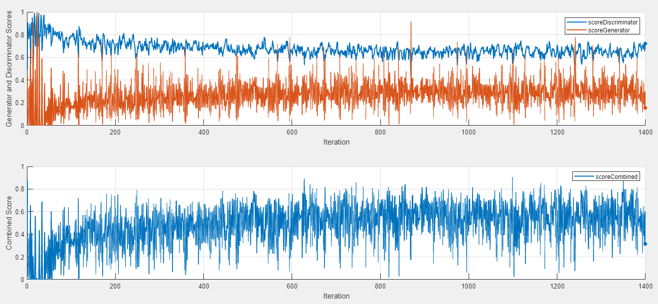
monitor.Metrics = ["scoreGenerator","scoreDiscriminator","scoreCombined"]; monitor.XLabel = "Iteration"; groupSubPlot(monitor,"Combined Score","scoreCombined"); groupSubPlot(monitor,"Generator and Discriminator Scores", ... ["scoreGenerator","scoreDiscriminator"]); monitor.Status = "Training";

augimdsTrain.MiniBatchSize = miniBatchSize; mbq = minibatchqueue(augimdsTrain,... MiniBatchSize=miniBatchSize,... PartialMiniBatch="discard",... MiniBatchFcn=@preprocessMiniBatch,... MiniBatchFormat="SSCB",... OutputEnvironment=output.executionEnvironment);

iteration = 0; for epoch = 1:numEpochs shuffle(mbq); while hasdata(mbq) iteration = iteration + 1; X = next(mbq);

    Z = randn(numLatentInputs,miniBatchSize,"single");
    Z = dlarray(Z,"CB");
    
    if (output.executionEnvironment == "auto" && canUseGPU) || ...
            output.executionEnvironment == "gpu"
        Z = gpuArray(Z);
    end
    
    [~,~,gradientsG,gradientsD,stateG,scoreG,scoreD] = ...
        dlfeval(@modelLoss,output.generator,output.discriminator,X,Z,flipFactor);
    output.generator.State = stateG;
    
    [output.discriminator,trailingAvgD,trailingAvgSqD] = adamupdate( ...
        output.discriminator,gradientsD, ...
        trailingAvgD,trailingAvgSqD,iteration, ...
        learnRate,gradientDecayFactor,squaredGradientDecayFactor);
    
    [output.generator,trailingAvgG,trailingAvgSqG] = adamupdate( ...
        output.generator,gradientsG, ...
        trailingAvgG,trailingAvgSqG,iteration, ...
        learnRate,gradientDecayFactor,squaredGradientDecayFactor);
    
    scoreG = double(gather(extractdata(scoreG)));
    scoreD = double(gather(extractdata(scoreD)));
    scoreCombinedValue = 1-2*max(abs(scoreD-0.5),abs(scoreG-0.5));
    
    recordMetrics(monitor,iteration, ...
        scoreGenerator=scoreG, ...
        scoreDiscriminator=scoreD, ...
        scoreCombined=scoreCombinedValue);
    
    if monitor.Stop || isnan(scoreG) || isnan(scoreD)
        return;
    end
end
monitor.Progress = (epoch/numEpochs)*100;

end

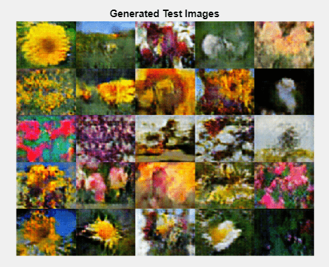
Generate Test Images creates a batch of 25 random vectors to input to the generator network and displays the resulting images in a figure. When the training is complete, the Review Results gallery in the toolstrip displays a button for the figure. The Name property of the figure specifies the name of the button. You can click the button to display the figure in the Visualizations pane. Use this figure to check that the generator produces a variety of images without many duplicates. If the images have little diversity and some of them are almost identical, then your generator is likely affected by mode collapse.

numLatentInputs = 100; numTestImages = 25;

ZTest = randn(numLatentInputs,numTestImages,"single"); ZTest = dlarray(ZTest,"CB");

if (output.executionEnvironment == "auto" && canUseGPU) || ... output.executionEnvironment == "gpu" ZTest = gpuArray(ZTest); end

XGenTest = predict(output.generator,ZTest);

figure(Name="Test Images") I = imtile(extractdata(XGenTest)); I = rescale(I); image(I) xticks([]) yticks([]) title("Generated Test Images")

Run Experiment

When you run the experiment, Experiment Manager trains the network defined by the training function multiple times. Each trial uses a different combination of hyperparameter values. By default, Experiment Manager runs one trial at a time. If you have Parallel Computing Toolbox, you can run multiple trials at the same time or offload your experiment as a batch job in a cluster:

To run one trial of the experiment at a time, on the Experiment Manager toolstrip, set Mode to Sequential and click Run.
To run multiple trials at the same time, set Mode to Simultaneous and click Run. If there is no current parallel pool, Experiment Manager starts one using the default cluster profile. Experiment Manager then runs as many simultaneous trials as there are workers in your parallel pool. For best results, before you run your experiment, start a parallel pool with as many workers as GPUs. For more information, see Run Experiments in Parallel and GPU Computing Requirements (Parallel Computing Toolbox).
To offload the experiment as a batch job, set Mode to Batch Sequential or Batch Simultaneous, specify your cluster and pool size, and click Run. For more information, see Offload Experiments as Batch Jobs to a Cluster.

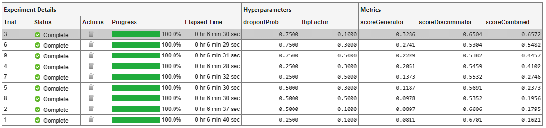
A table of results displays the training loss and validation accuracy for each trial.

To display the training plot and track the progress of each trial while the experiment is running, under Review Results, click Training Plot.

Evaluate Results

Training GANs can be a challenging task because the generator and the discriminator networks compete against each other during the training. If one network learns too quickly, then the other network can fail to learn. To help you diagnose issues and monitor how well the generator and discriminator networks achieve their respective goals, this experiment displays a pair of scores in the training plot. The generator score scoreGenerator measures the likelihood that the discriminator can correctly distinguish generated images. The discriminator score scoreDiscriminator measures the likelihood that the discriminator can correctly distinguish all input images, assuming that the numbers of real and generated images passed to the discriminator are equal. In the ideal case, both scores are 0.5. Scores that are too close to zero or one can indicate that one network dominates the other. For more information, see Monitor GAN Training Progress and Identify Common Failure Modes.

To help you decide which trial produces the best results, this experiment combines the generator score and discriminator scores into a single numeric value, scoreCombined. This metric uses the _L_-∞ norm to determine how close the two networks are to the ideal scenario. The metric returns a value of one if both network scores equal 0.5, and zero if one of the network scores equals zero or one. To sort the table of results using the combined score:

Point to the scoreCombined column.
Click the triangle icon.
Select Sort in Descending Order.

The trial with the highest combined score appears at the top of the results table.

Using the combined score to sort your results might not identify the best trial in all cases. To evaluate the quality of the GAN, inspect the images produced by the trained generator. First, select a row in the results table. Then, on the Experiment Manager toolstrip, under Review Results, click Test Images. Experiment Manager displays the images generated from a batch of 25 random vectors.

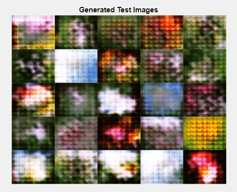
For best results, repeat this process for each trial with a high combined score to visually check that the generator produces a variety of images without many duplicates. If the images have little diversity and some of them are almost identical, then your generator is likely affected by mode collapse. For more information, see Mode Collapse.

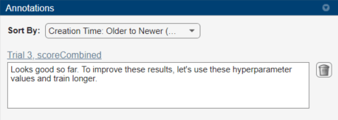
To record observations about the results of your experiment, add an annotation:

In the results table, right-click the scoreCombined cell for the best trial.
Select Add Annotation.
In the Annotations pane, enter your observations in the text box.

Rerun Experiment

After you identify the combination of hyperparameters that generates the best images, run the experiment a second time to train the network for a longer period of time:

Return to the experiment definition tab.
In the hyperparameter table, enter the hyperparameter values from your best trial. For example, to use the values from trial 3, change the value of dropoutProb to 0.75 and flipFactor to 0.1.
Open the training function and specify a longer training time. Under Specify Training Options, change the value of numEpochs to 500.
Run the experiment using the new hyperparameter values and training function. Experiment Manager runs a single trial. Training takes about 10 times longer than the previous trials.
When the experiment finishes, test the new generator network by inspecting the generated test images. As before, visually check that the generator produces a variety of images without many duplicates.

Close Experiment

In the Experiment Browser pane, right-click FlowerImageGenerationProject and select Close Project. Experiment Manager closes the experiment and results contained in the project.

Training Function

This function specifies the training data, network architecture, training options, and training procedure used by the experiment. The input to this function is a structure with fields from the hyperparameter table and an experiments.Monitor object that you can use to track the progress of the training, record values of the metrics used by the training, and produce training plots. The training function returns a structure that contains the trained generator network, the trained discriminator network, and the execution environment used for training. Experiment Manager saves this output so you can export it to the MATLAB workspace when the training is complete.

function output = ImageGenerationExperiment_training(params,monitor)

Initialize Output

output.generator = []; output.discriminator = []; output.executionEnvironment = "auto";

Load Training Data

monitor.Status = "Loading Data";

url = "http://download.tensorflow.org/example_images/flower_photos.tgz"; downloadFolder = tempdir; filename = fullfile(downloadFolder,"flower_dataset.tgz");

imageFolder = fullfile(downloadFolder,"flower_photos"); if ~exist(imageFolder,"dir") websave(filename,url); untar(filename,downloadFolder) end

datasetFolder = fullfile(imageFolder); imdsTrain = imageDatastore(datasetFolder, ... IncludeSubfolders=true);

augmenter = imageDataAugmenter(RandXReflection=true); augimdsTrain = augmentedImageDatastore([64 64],imdsTrain, ... DataAugmentation=augmenter);

Define Generator Network

monitor.Status = "Creating Generator";

filterSize = 5; numFilters = 64; numLatentInputs = 100; projectionSize = [4 4 512];

lgraphGenerator = layerGraph(layersGenerator); output.generator = dlnetwork(lgraphGenerator);

Define Discriminator Network

monitor.Status = "Creating Discriminator";

filterSize = 5; numFilters = 64; inputSize = [64 64 3]; dropoutProb = params.dropoutProb; scale = 0.2;

lgraphDiscriminator = layerGraph(layersDiscriminator); output.discriminator = dlnetwork(lgraphDiscriminator);

Specify Training Options

Train Model

iteration = 0; for epoch = 1:numEpochs shuffle(mbq); while hasdata(mbq) iteration = iteration + 1; X = next(mbq);

    Z = randn(numLatentInputs,miniBatchSize,"single");
    Z = dlarray(Z,"CB");
    
    if (output.executionEnvironment == "auto" && canUseGPU) || ...
            output.executionEnvironment == "gpu"
        Z = gpuArray(Z);
    end
    
    [~,~,gradientsG,gradientsD,stateG,scoreG,scoreD] = ...
        dlfeval(@modelLoss,output.generator,output.discriminator,X,Z,flipFactor);
    output.generator.State = stateG;
    
    [output.discriminator,trailingAvgD,trailingAvgSqD] = adamupdate( ...
        output.discriminator,gradientsD, ...
        trailingAvgD,trailingAvgSqD,iteration, ...
        learnRate,gradientDecayFactor,squaredGradientDecayFactor);
    
    [output.generator,trailingAvgG,trailingAvgSqG] = adamupdate( ...
        output.generator,gradientsG, ...
        trailingAvgG,trailingAvgSqG,iteration, ...
        learnRate,gradientDecayFactor,squaredGradientDecayFactor);
    
    scoreG = double(gather(extractdata(scoreG)));
    scoreD = double(gather(extractdata(scoreD)));
    scoreCombinedValue = 1-2*max(abs(scoreD-0.5),abs(scoreG-0.5));
    
    recordMetrics(monitor,iteration, ...
        scoreGenerator=scoreG, ...
        scoreDiscriminator=scoreD, ...
        scoreCombined=scoreCombinedValue);
    
    if monitor.Stop || isnan(scoreG) || isnan(scoreD)
        return;
    end
end
monitor.Progress = (epoch/numEpochs)*100;

end

Generate Test Images

numLatentInputs = 100; numTestImages = 25;

ZTest = randn(numLatentInputs,numTestImages,"single"); ZTest = dlarray(ZTest,"CB");

if (output.executionEnvironment == "auto" && canUseGPU) || ... output.executionEnvironment == "gpu" ZTest = gpuArray(ZTest); end

XGenTest = predict(output.generator,ZTest);

figure(Name="Test Images") I = imtile(extractdata(XGenTest)); I = rescale(I); image(I) xticks([]) yticks([]) title("Generated Test Images")

Helper Functions

The modelLoss function takes as input the generator and discriminator dlnetwork objects (netG and netD), a mini-batch of input data (X), an array of random values (Z), and the percentage of real labels to flip (flipProb), and returns the loss values, the gradients of the loss values with respect to the learnable parameters in the networks, the generator state, and the scores of the two networks.

function [lossG,lossD,gradientsG,gradientsD,stateG,scoreG,scoreD] = ... modelLoss(netG,netD,X,Z,flipProb)

YReal = forward(netD,X);

[XGenerated,stateG] = forward(netG,Z); YGenerated = forward(netD,XGenerated);

scoreD = (mean(YReal) + mean(1-YGenerated)) / 2; scoreG = mean(YGenerated);

numObservations = size(YReal,4); idx = rand(1,numObservations) < flipProb; YReal(:,:,:,idx) = 1 - YReal(:,:,:,idx);

[lossG, lossD] = GANLoss(YReal,YGenerated);

gradientsG = dlgradient(lossG,netG.Learnables,RetainData=true); gradientsD = dlgradient(lossD,netD.Learnables); end

The GANLoss function returns the loss for the discriminator and generator networks.

function [lossG,lossD] = GANLoss(YReal,YGenerated) lossD = -mean(log(YReal))-mean(log(1-YGenerated)); lossG = -mean(log(YGenerated)); end

The preprocessMiniBatch function preprocesses the data by extracting the image data from the incoming cell array, concatenating the images into a numeric array, and rescaling the images to be in the range [-1,1].

function X = preprocessMiniBatch(data) X = cat(4,data{:}); X = rescale(X,-1,1,InputMin=0,InputMax=255); end

Use Experiment Manager to Train Generative Adversarial Networks (GANs) - MATLAB & Simulink (original) (raw)

Open Experiment

Run Experiment

Evaluate Results

Rerun Experiment

Close Experiment

Training Function

Helper Functions

See Also

Apps

Objects

Topics