Perform Calculations by Group in Table - MATLAB & Simulink (original) (raw)
Main Content
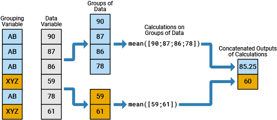
You can perform calculations on groups of data within table variables. In such calculations, you split one or more table variables into groups of data, perform a calculation on each group, and combine the results into one or more output variables. MATLAB® provides several functions that split data into groups and combine the results for you. You need only specify which table variables contain data, which variables define groups, and the function to apply to the groups of data.
For example, this diagram shows a simple grouped calculation that splits a numeric table variable into two groups of data, calculates the mean of each group, and then combines the mean values into an output variable.
You can perform grouped calculations on table variables by using any of methods in this list:
groupsummary,groupcounts,groupfilter, andgrouptransformvarfunandrowfunfindgroupsandsplitapply- Compute by Group task in the Live Editor
In most cases, groupsummary is the recommended function for grouped calculations. It is simple to use and returns a table with labels that describe results. The other listed functions, however, also offer capabilities that can be useful in some situations.
This topic has examples that use each of these functions. It ends with a summary of their behaviors and recommended usages.
Create Table from File
The sample spreadsheet outages.csv contains data values that represent electric utility power outages in the United States. To create a table from the file, use the readtable function. To read text data from the file into table variables that are string arrays, specify the TextType name-value argument as "string".
outages = readtable("outages.csv","TextType","string")
outages=1468×6 table
Region OutageTime Loss Customers RestorationTime Cause
___________ ________________ ______ __________ ________________ _________________
"SouthWest"    2002-02-01 12:18    458.98    1.8202e+06    2002-02-07 16:50    "winter storm"
"SouthEast"    2003-01-23 00:49    530.14    2.1204e+05                 NaT    "winter storm"
"SouthEast"    2003-02-07 21:15     289.4    1.4294e+05    2003-02-17 08:14    "winter storm"
"West"         2004-04-06 05:44    434.81    3.4037e+05    2004-04-06 06:10    "equipment fault"
"MidWest"      2002-03-16 06:18    186.44    2.1275e+05    2002-03-18 23:23    "severe storm"
"West"         2003-06-18 02:49         0             0    2003-06-18 10:54    "attack"
"West"         2004-06-20 14:39    231.29           NaN    2004-06-20 19:16    "equipment fault"
"West"         2002-06-06 19:28    311.86           NaN    2002-06-07 00:51    "equipment fault"
"NorthEast"    2003-07-16 16:23    239.93         49434    2003-07-17 01:12    "fire"
"MidWest"      2004-09-27 11:09    286.72         66104    2004-09-27 16:37    "equipment fault"
"SouthEast"    2004-09-05 17:48    73.387         36073    2004-09-05 20:46    "equipment fault"
"West"         2004-05-21 21:45    159.99           NaN    2004-05-22 04:23    "equipment fault"
"SouthEast"    2002-09-01 18:22    95.917         36759    2002-09-01 19:12    "severe storm"
"SouthEast"    2003-09-27 07:32       NaN    3.5517e+05    2003-10-04 07:02    "severe storm"
"West"         2003-11-12 06:12    254.09    9.2429e+05    2003-11-17 02:04    "winter storm"
"NorthEast"    2004-09-18 05:54         0             0                 NaT    "equipment fault"
  ⋮
Create categorical Grouping Variables
Table variables can have any data type. But conceptually, you can also think of tables as having two general kinds of variables: data variables and grouping variables.
- Data variables enable you to describe individual events or observations. For example, in
outagesyou can think of theOutageTime,Loss,Customers, andRestorationTimevariables as data variables. - Grouping variables enable you to group together events or observations that have something in common. For example, in
outagesyou can think of theRegionandCausevariables as grouping variables. You can group together and analyze the power outages that occur in the same region or share the same cause.
Often, grouping variables contain a discrete set of fixed values that specify categories. The categories specify groups that data values can belong to. The categorical data type can be a convenient type for working with categories.
To convert Region and Cause to categorical variables, use the convertvars function.
outages = convertvars(outages,["Region","Cause"],"categorical")
outages=1468×6 table
Region OutageTime Loss Customers RestorationTime Cause
_________ ________________ ______ __________ ________________ _______________
SouthWest    2002-02-01 12:18    458.98    1.8202e+06    2002-02-07 16:50    winter storm
SouthEast    2003-01-23 00:49    530.14    2.1204e+05                 NaT    winter storm
SouthEast    2003-02-07 21:15     289.4    1.4294e+05    2003-02-17 08:14    winter storm
West         2004-04-06 05:44    434.81    3.4037e+05    2004-04-06 06:10    equipment fault
MidWest      2002-03-16 06:18    186.44    2.1275e+05    2002-03-18 23:23    severe storm
West         2003-06-18 02:49         0             0    2003-06-18 10:54    attack
West         2004-06-20 14:39    231.29           NaN    2004-06-20 19:16    equipment fault
West         2002-06-06 19:28    311.86           NaN    2002-06-07 00:51    equipment fault
NorthEast    2003-07-16 16:23    239.93         49434    2003-07-17 01:12    fire
MidWest      2004-09-27 11:09    286.72         66104    2004-09-27 16:37    equipment fault
SouthEast    2004-09-05 17:48    73.387         36073    2004-09-05 20:46    equipment fault
West         2004-05-21 21:45    159.99           NaN    2004-05-22 04:23    equipment fault
SouthEast    2002-09-01 18:22    95.917         36759    2002-09-01 19:12    severe storm
SouthEast    2003-09-27 07:32       NaN    3.5517e+05    2003-10-04 07:02    severe storm
West         2003-11-12 06:12    254.09    9.2429e+05    2003-11-17 02:04    winter storm
NorthEast    2004-09-18 05:54         0             0                 NaT    equipment fault
  ⋮
Calculate Statistics by Group in Table
You can calculate statistics by group in a table using functions such as groupsummary, varfun, and splitapply. These functions enable you to specify groups of data within a table and methods that perform calculations on each group. You can store the results in another table or in output arrays.
For example, determine the mean power loss and customers affected due to the outages in each region in the outages table. The recommended way to perform this calculation is to use the groupsummary function. Specify Region as the grouping variable, mean as the method to apply to each group, and Loss and Customers as the data variables. The output lists the regions (in the Region variable), the number of power outages per region (in the GroupCount variable), and the mean power loss and customers affected in each region (in the mean_Loss and mean_Customers variables, respectively).
meanLossByRegion = groupsummary(outages,"Region","mean",["Loss","Customers"])
meanLossByRegion=5×4 table Region GroupCount mean_Loss mean_Customers _________ __________ _________ ______________
MidWest         142         1137.7        2.4015e+05
NorthEast       557         551.65        1.4917e+05
SouthEast       389         495.35        1.6776e+05
SouthWest        26         493.88        2.6975e+05
West            354         433.37        1.5201e+05
The groupsummary function is recommended for several reasons:
- You can specify many common methods (such as
max,min, andmean) by name, without using function handles. - You can specify multiple methods in one call.
NaNs,NaTs, and other missing values in the data variables are automatically omitted when calculating results.
The third point explains why the mean_Loss and mean_Customers variables do not have NaNs in the meanLossByRegion output table.
To specify multiple methods in one call to groupsummary, list them in an array. For example, calculate the maximum, mean, and minimum power loss by region.
lossStatsByRegion = groupsummary(outages,"Region",["max","mean","min"],"Loss")
lossStatsByRegion=5×5 table Region GroupCount max_Loss mean_Loss min_Loss _________ __________ ________ _________ ________
MidWest         142          23141      1137.7         0
NorthEast       557          23418      551.65         0
SouthEast       389         8767.3      495.35         0
SouthWest        26           2796      493.88         0
West            354          16659      433.37         0
The minimum loss in every region is zero. To analyze only those outages that resulted in losses greater than zero, exclude the rows in outages where the loss is zero. First create a vector of logical indices whose values are logical 1 (true) for rows where outages.Loss is greater than zero. Then index into outages to return a table that includes only those rows. Again, calculate the maximum, mean, and minimum power loss by region.
nonZeroLossIndices = outages.Loss > 0; nonZeroLossOutages = outages(nonZeroLossIndices,:); nonZeroLossStats = groupsummary(nonZeroLossOutages,"Region",["max","mean","min"],"Loss")
nonZeroLossStats=5×5 table Region GroupCount max_Loss mean_Loss min_Loss _________ __________ ________ _________ ________
MidWest          81          23141      1264.1       8.9214
NorthEast       180          23418      827.47      0.74042
SouthEast       234         8767.3      546.16       2.3096
SouthWest        23           2796      515.35       27.882
West            175          16659      549.76      0.71847
Use Alternative Functions for Grouped Calculations
There are alternative functions that perform grouped calculations in tables. While groupsummary is recommended, the alternative functions are also useful in some situations.
- The
varfunfunction performs calculations on variables. It is similar togroupsummary, butvarfuncan perform both grouped and ungrouped calculations. - The
rowfunfunction performs calculations along rows. You can specify methods that take multiple inputs or that return multiple outputs. - The
findgroupsandsplitapplyfunctions can perform calculations on variables or along rows. You can specify methods that take multiple inputs or that return multiple outputs. The outputs ofsplitapplyare arrays, not tables.
Call varfun on Variables
For example, calculate the maximum power loss by region using varfun. The output table has a similar format to the output of groupsummary.
maxLossByVarfun = varfun(@max, ... outages, ... "InputVariables","Loss", ... "GroupingVariables","Region")
maxLossByVarfun=5×3 table Region GroupCount max_Loss _________ __________ ________
MidWest         142          23141
NorthEast       557          23418
SouthEast       389         8767.3
SouthWest        26           2796
West            354          16659
However, there are significant differences when you use varfun:
- You must always specify the method by using a function handle.
- You can specify only one method.
- You can perform grouped or ungrouped calculations.
NaNs,NaTs, and other missing values in the data variables are automatically included when calculating results.
The last point is a significant difference in behavior between groupsummary and varfun. For example, the Loss variable has NaNs. If you use varfun to calculate the mean losses, then by default the results are NaNs, unlike the default groupsummary results.
meanLossByVarfun = varfun(@mean, ... outages, ... "InputVariables","Loss", ... "GroupingVariables","Region")
meanLossByVarfun=5×3 table Region GroupCount mean_Loss _________ __________ _________
MidWest         142           NaN
NorthEast       557           NaN
SouthEast       389           NaN
SouthWest        26           NaN
West            354           NaN
To omit missing values when using varfun, wrap the method in an anonymous function so that you can specify the "omitnan" option.
omitnanMean = @(x)(mean(x,"omitnan"));
meanLossOmitNaNs = varfun(omitnanMean, ... outages, ... "InputVariables","Loss", ... "GroupingVariables","Region")
meanLossOmitNaNs=5×3 table Region GroupCount Fun_Loss _________ __________ ________
MidWest         142         1137.7
NorthEast       557         551.65
SouthEast       389         495.35
SouthWest        26         493.88
West            354         433.37
Another point refers to a different but related use case, which is to perform ungrouped calculations on table variables. To apply a method to all table variables without grouping, use varfun. For example, calculate the maximum power loss and the maximum number of customers affected in the entire table.
maxValuesInOutages = varfun(@max, ... outages, ... "InputVariables",["Loss","Customers"])
maxValuesInOutages=1×2 table max_Loss max_Customers ________ _____________
23418 5.9689e+06 Call rowfun on Rows
The rowfun function applies a method along the rows of a table. Where varfun applies a method to each specified variable, one by one, rowfun takes all specified table variables as input arguments to the method and applies the method once.
For example, calculate the median loss per customer in each region. To perform this calculation, first specify a function that takes two input arguments (loss and customers), divides the loss by the number of customers, and then returns the median.
medianLossCustFcn = @(loss,customers)(median(loss ./ customers,"omitnan"));
Then call rowfun. You can specify a meaningful output variable name by using the OutputVariablesNames name-value argument.
meanLossPerCustomer = rowfun(medianLossCustFcn, ... outages, ... "InputVariables",["Loss","Customers"], ... "GroupingVariables","Region", ... "OutputVariableNames","MedianLossPerCustomer")
meanLossPerCustomer=5×3 table Region GroupCount MedianLossPerCustomer _________ __________ _____________________
MidWest         142              0.0042139
NorthEast       557              0.0028512
SouthEast       389              0.0032057
SouthWest        26              0.0026353
West            354               0.002527
You can also use rowfun when the method returns multiple outputs. For example, use bounds to calculate the minimum and maximum loss per region in one call to rowfun. The bounds function returns two output arguments.
boundsLossPerRegion = rowfun(@bounds, ... outages, ... "InputVariables","Loss", ... "GroupingVariables","Region", ... "OutputVariableNames",["MinLoss","MaxLoss"])
boundsLossPerRegion=5×4 table Region GroupCount MinLoss MaxLoss _________ __________ _______ _______
MidWest         142           0        23141
NorthEast       557           0        23418
SouthEast       389           0       8767.3
SouthWest        26           0         2796
West            354           0        16659
Call findgroups and splitapply on Variables or Rows
You can use the findgroups function to define groups and then use splitapply to apply a method to each group. The findgroups function returns a vector of group numbers that identifies which group a row of data is part of. The splitapply function returns a numeric array of the outputs of the method applied to the groups.
For example, calculate the maximum power loss by region using findgroups and splitapply.
G = findgroups(outages.Region)
G = 1468×1
 4
 3
 3
 5
 1
 5
 5
 5
 2
 1
 3
 5
 3
 3
 5
  ⋮
maxLossArray = splitapply(@max,outages.Loss,G)
maxLossArray = 5×1 104 ×
2.3141
2.3418
0.8767
0.2796
1.6659
Like rowfun, splitapply enables you to specify methods that return multiple outputs. Calculate both minima and maxima by using bounds.
[minLossArray,maxLossArray] = splitapply(@bounds,outages.Loss,G)
minLossArray = 5×1
 0
 0
 0
 0
 0
maxLossArray = 5×1 104 ×
2.3141
2.3418
0.8767
0.2796
1.6659
You can also specify methods that take multiple inputs. For example, use the medianLossCustFcn function again to calculate the median loss per customer. But this time, return the median loss per customer in each region as an array.
medianLossCustFcn = @(loss,customers)(median(loss ./ customers,"omitnan"));
medianLossArray = splitapply(medianLossCustFcn,outages.Loss,outages.Customers,G)
medianLossArray = 5×1
0.0042
0.0029
0.0032
0.0026
0.0025
The numeric outputs of findgroups and splitapply are not annotated like the output of groupsummary. However, returning numeric outputs can have other benefits:
- You can use the output of
findgroupsin multiple calls tosplitapply. You might want to usefindgroupsandsplitapplyfor efficiency when you make many grouped calculations on a large table. - You can create a results table with a different format by building it from the outputs of
findgroupsandsplitapply. - You can call methods that return multiple outputs.
- You can append the outputs of
splitapplyto an existing table.
Append New Calculation to Existing Table
If you already have a table of results, you can append the results of another calculation to that table. For example, calculate the mean duration of power outages in each region in hours. Append the mean durations as a new variable to the lossStatsByRegion table.
First subtract the outage times from the restoration times to return the durations of the power outages. Convert these durations to hours by using the hours function.
D = outages.RestorationTime - outages.OutageTime; H = hours(D)
H = 1468×1 105 ×
0.0015
   NaN
0.0023
0.0000
0.0007
0.0001
0.0000
0.0001
0.0001
0.0001
0.0000
0.0001
0.0000
0.0017
0.0012
  ⋮
Next use mean to calculate the mean durations. The outage durations have some NaN values because the outage and restoration times have some missing values. As before, wrap the method in an anonymous function to specify the "omitnan" option.
omitnanMean = @(x)(mean(x,"omitnan"));
Calculate the mean duration of power outages by region. Append it to lossStatsByRegion as a new table variable.
G = findgroups(outages.Region); lossStatsByRegion.mean_Outage = splitapply(omitnanMean,H,G)
lossStatsByRegion=5×6 table Region GroupCount max_Loss mean_Loss min_Loss mean_Outage _________ __________ ________ _________ ________ ___________
MidWest         142          23141      1137.7         0          819.25
NorthEast       557          23418      551.65         0          581.04
SouthEast       389         8767.3      495.35         0           40.83
SouthWest        26           2796      493.88         0          59.519
West            354          16659      433.37         0          673.45
Specify Groups as Bins
There is another way to specify groups. Instead of specifying categories as unique values in a grouping variable, you can bin values in a variable where values are distributed continuously. Then you can use those bins to specify groups.
For example, bin the power outages by year. To count the number of power outages per year, use the groupcounts function.
outagesByYear = groupcounts(outages,"OutageTime","year")
outagesByYear=13×3 table year_OutageTime GroupCount Percent _______________ __________ _______
     2002              36         2.4523
     2003              62         4.2234
     2004              79         5.3815
     2005              74         5.0409
     2006             108         7.3569
     2007              91         6.1989
     2008             115         7.8338
     2009             142          9.673
     2010             177         12.057
     2011             190         12.943
     2012             207         14.101
     2013             186          12.67
     2014               1        0.06812
Visualize the number of outages per year. The number per year increases over time in this data set.
bar(outagesByYear.year_OutageTime,outagesByYear.GroupCount)

You can use groupsummary with bins as groups. For example, calculate the median values for customers affected and power losses by year.
medianLossesByYear = groupsummary(outages,"OutageTime","year","median",["Customers","Loss"])
medianLossesByYear=13×4 table year_OutageTime GroupCount median_Customers median_Loss _______________ __________ ________________ ___________
     2002              36           1.7101e+05         277.02
     2003              62           1.0204e+05          295.6
     2004              79           1.0108e+05         252.44
     2005              74                91536         265.16
     2006             108                86020         210.08
     2007              91           1.0529e+05         232.12
     2008             115                86356         205.77
     2009             142                63119         83.491
     2010             177                66212         155.76
     2011             190                48200         75.286
     2012             207                66994         78.289
     2013             186                55669         69.596
     2014               1                  NaN            NaN
Visualize the median number of customers affected by outages per year. Although the number of outages increased over time, the median number of affected customers decreased.
plot(medianLossesByYear,"year_OutageTime","median_Customers")

Return the rows of outages for years with more than 75 outages. To index into outages by those years, use the groupfilter function. To find the bins with more than 75 rows, specify an anonymous function that returns a logical 1 if the number of rows in a bin is greater than 75.
outages75 = groupfilter(outages,"OutageTime","year",@(x) numel(x) > 75)
outages75=1295×7 table Region OutageTime Loss Customers RestorationTime Cause year_OutageTime _________ ________________ ______ __________ ________________ _______________ _______________
West         2004-04-06 05:44    434.81    3.4037e+05    2004-04-06 06:10    equipment fault         2004
West         2004-06-20 14:39    231.29           NaN    2004-06-20 19:16    equipment fault         2004
MidWest      2004-09-27 11:09    286.72         66104    2004-09-27 16:37    equipment fault         2004
SouthEast    2004-09-05 17:48    73.387         36073    2004-09-05 20:46    equipment fault         2004
West         2004-05-21 21:45    159.99           NaN    2004-05-22 04:23    equipment fault         2004
NorthEast    2004-09-18 05:54         0             0                 NaT    equipment fault         2004
NorthEast    2004-11-13 10:42       NaN    1.4227e+05    2004-11-19 02:31    winter storm            2004
SouthEast    2004-12-06 23:18       NaN         37136    2004-12-14 03:21    winter storm            2004
West         2004-12-21 18:50    112.05     7.985e+05    2004-12-29 03:46    winter storm            2004
NorthEast    2004-12-26 22:18    255.45    1.0444e+05    2004-12-27 14:11    winter storm            2004
SouthWest    2004-06-06 05:27    559.41      2.19e+05    2004-06-06 05:55    equipment fault         2004
MidWest      2004-07-02 09:16     15128    2.0104e+05    2004-07-06 14:11    thunder storm           2004
SouthWest    2004-07-18 14:40    340.35    1.4963e+05    2004-07-26 23:34    severe storm            2004
NorthEast    2004-09-16 19:42      4718           NaN                 NaT    unknown                 2004
SouthEast    2004-09-20 12:37    8767.3    2.2249e+06    2004-10-02 06:00    severe storm            2004
MidWest      2004-11-09 18:44    470.83         67587    2004-11-09 21:24    wind                    2004
  ⋮
Summary of Behavior and Recommendations
Use these tips and recommendations to decide which functions to use to perform group calculations.
- Specify groups using either grouping variables or bins created from numeric,
datetime, ordurationvariables. - To perform calculations by group on data in tables or timetables, use the recommended function
groupsummary. The related functionsgroupcounts,groupfilter, andgrouptransformalso are useful. - Consider using
varfunto automatically include missing values (such asNaNs andNaTs) when applying methods to groups of data. Also,varfuncan perform both grouped and ungrouped calculations. - Consider using
findgroupsandsplitapplyfor efficiency when you make many consecutive grouped calculations on a large table. - Consider using
findgroupsandsplitapplyto append new arrays to an existing table of results. - To perform calculations using a method that returns multiple outputs, such as
bounds, use eitherrowfunorsplitapply. - To perform calculations along rows using a method that requires multiple input arguments, use either
rowfunorsplitapply.
See Also
groupsummary | groupcounts | groupfilter | grouptransform | varfun | rowfun | findgroups | splitapply | table | categorical | datetime | duration | readtable | convertvars | bounds