Optimize parfor-Loops with Pool Dashboard - MATLAB & Simulink (original) (raw)
This example shows how to use pool monitoring data from the Pool Dashboard to optimize a parfor-loop.
The Pool Dashboard is a tool that provides a visual interface to monitor and optimize parallel tasks. You can visualize the distribution of workloads across workers to help you optimize your parallel code.
In this example, you use a parfor-loop to process a collection of images by computing their fast Fourier transform (FFT). The computational load for each image depends on its file size, which can vary significantly. Use the Pool Dashboard to understand the workload distribution across the workers and identify any bottlenecks in the parfor-loop.
Set Up Pool and Create Image Files
Create a parallel pool using the parpool function. By default, parpool uses your default profile. Check your default profile on the MATLAB Home tab, in Parallel > Select Parallel Environment.
Starting parallel pool (parpool) using the 'Processes' profile ... Connected to parallel pool with 6 workers.
Create a collection of image files for analysis using the createFiles helper function, which is defined at the end of this example.
Obtain a list of the image filenames and extract the number of images. Preallocate a structure for the results data.
imageFiles = dir("images/*.jpg"); numImages = numel(imageFiles); outputSpectra = struct("scanNumber",[],"spectra",[]);
Open Pool Dashboard
To open the Pool Dashboard, select one of these options:
- MATLAB® Toolstrip: On the Home tab in the Environment section, select Parallel > Open Pool Dashboard.
- Parallel status indicator: Click the indicator icon and select Open Pool Dashboard.
- MATLAB command prompt: Enter
parpoolDashboard.
Collect Pool Monitoring Data for Image Processing with parfor
Process the collection of images by computing their FFT. Use a parfor-loop to accelerate image processing with the fftImage helper function, which is defined at the end of this example.
Collect monitoring data with the Pool Dashboard. In the Monitoring section of the Pool Dashboard, select Start Monitoring. When the Pool Dashboard begins collecting monitoring data, return to the Live Editor and click Run Section.
 parfor idx = 1:numImages
imgName = imageFiles(idx).name;
outputSpectra(idx) = fftImage(imgName);
end
parfor idx = 1:numImages
imgName = imageFiles(idx).name;
outputSpectra(idx) = fftImage(imgName);
end
disp("Section complete.")
After the section code is complete, in the Monitoring section of the Pool Dashboard, select Stop. The Pool Dashboard displays the monitoring results.
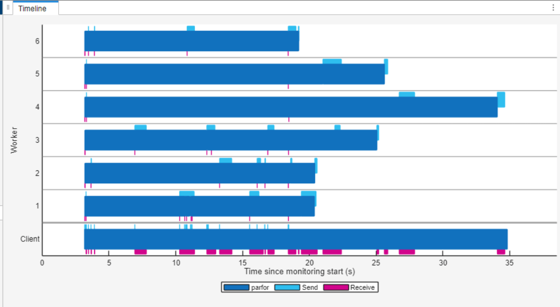
To review the monitoring data, focus on the Timeline graph. The Timeline graph visually represents the time workers and the client spend running the parfor-loop and transferring data. Dark blue indicates the time spent running the parfor-loop, while light blue represents sending data and magenta represents receiving data. You can observe that workers 3, 4 and 5 take significantly longer to process the images the parfor function assigns to them compared to the other workers. This observation suggests that the load is not evenly distributed across the workers.
Optimize parfor Load Distribution
You can use different approaches to optimize the load distribution for the parfor-loop. This section discusses how to achieve a more balanced workload distribution both when the workload of each iteration is unknown and when it is known.
Randomize Files
If you do not have any information about the workload of each iteration, randomizing the order of processing can help balance the workload. To process the images in a random order, use the randperm function to generate a random permutation of indices for the image files.
Collect monitoring data with the Pool Dashboard, in the Monitoring section of the Pool Dashboard, select Start Monitoring. When the Pool Dashboard begins collecting monitoring data, return to the Live Editor and click Run Section.
 randIndices = randperm(numImages);
randImageFiles = imageFiles(randIndices);
parfor idx = 1:numImages
imgName = randImageFiles(idx).name;
outputSpectra(idx) = fftImage(imgName);
end
disp("Section complete")
randIndices = randperm(numImages);
randImageFiles = imageFiles(randIndices);
parfor idx = 1:numImages
imgName = randImageFiles(idx).name;
outputSpectra(idx) = fftImage(imgName);
end
disp("Section complete")
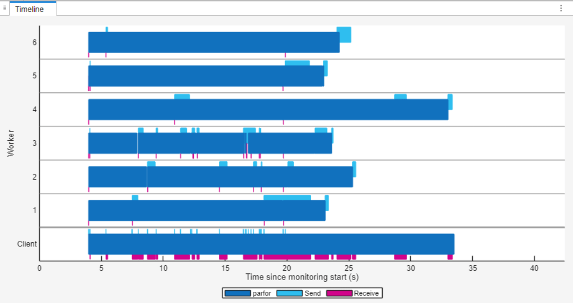
After the section code is complete, in the Monitoring section of the Pool Dashboard, select Stop. In the Timeline graph, you can observe that the workers are idle for less time compared to the first parfor-loop. This observation indicates that the load distribution is more balanced than before.
Control parfor Range Partitioning
In a parfor-loop, a subrange is a contiguous block of loop iterations executed as a group on a worker. You can control how parfor partitions these iterations into subranges using the parforOptions function. For more information, see parforOptions.
For optimal performance, aim to create subranges that are:
- Large enough so that the computation time is substantial compared to the overhead of scheduling the subrange
- Small enough to ensure there are enough subranges to keep all workers busy
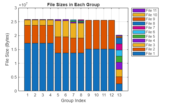
In this example, the computational load for each image depends on its size. To partition iterations more effectively, you can calculate subranges based on the file sizes. The groupImageFilesBySize helper function groups the image files by their sizes, using an upper limit of 1.5 times the size of the largest image file for the cumulative size of the files in each group. The groupImageFilesBySize function is attached to this example as a supporting file.
[subranges,groupedImageFiles] = groupImageFilesBySize(imageFiles);
To understand how the groupImageFilesBySize function groups the images, view the distribution of file sizes in the groups in a bar chart.
barSubranges(groupedImageFiles,subranges);
To run a parfor-loop using the calculated subranges, pass a function handle to the 'RangePartitionMethod' name-value argument. This function handle must return a vector of subrange sizes, and their sum must be equal to the number of iterations.
opts = parforOptions(pool,RangePartitionMethod=@(n,nw) subranges);
To collect monitoring data with the Pool Dashboard, in the Monitoring section, select Start Monitoring. When the Pool Dashboard begins collecting monitoring data, return to the Live Editor and click Run Section.
 parfor (idx = 1:numImages,opts)
imgName = groupedImageFiles(idx).name;
outputSpectra(idx) = fftImage(imgName);
end
disp("Section complete")
parfor (idx = 1:numImages,opts)
imgName = groupedImageFiles(idx).name;
outputSpectra(idx) = fftImage(imgName);
end
disp("Section complete")
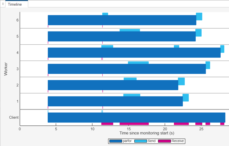
After the section code is complete, in the Monitoring section of the Pool Dashboard, select Stop. In the Timeline graph, you can observe that almost all of the workers are idle for less time compared to the first parfor-loop. The parfor-loop also completes in less time.
Convert parfor-Loop to parfeval Computations
An alternative to using parfor for parallel processing is the parfeval function. With parfeval, you can schedule the evaluation of a function on a pool worker for each iteration. This approach provides more flexibility for scheduling work on the workers and can help prevent workers from remaining idle, as each worker is assigned one iteration at a time and can perform other tasks if no new parfeval computations are pending.
For each image, you schedule a call to the fftImage helper function using parfeval. The software queues each function call for execution on a worker in the parallel pool. Unlike parfor, which divides the iterations into subranges, parfeval allows you to manage each task individually.
To collect monitoring data with the Pool Dashboard, in the Monitoring section, select Start Monitoring. When the Pool Dashboard begins collecting monitoring data, return to the Live Editor and click Run Section.
 futures(1:numImages) = parallel.Future;
for idx = 1:numImages
imgName = imageFiles(idx).name;
futures(idx) = parfeval(@fftImage,1,imgName);
end
futures(1:numImages) = parallel.Future;
for idx = 1:numImages
imgName = imageFiles(idx).name;
futures(idx) = parfeval(@fftImage,1,imgName);
end
As each task completes, you can retrieve the results using the fetchNext function. fetchNext returns the index of the completed task and its output, allowing you to store the results in the correct order.
for idx = 1:numImages [resultIdx,output] = fetchNext(futures); outputSpectra(resultIdx) = output; end disp("Section complete")
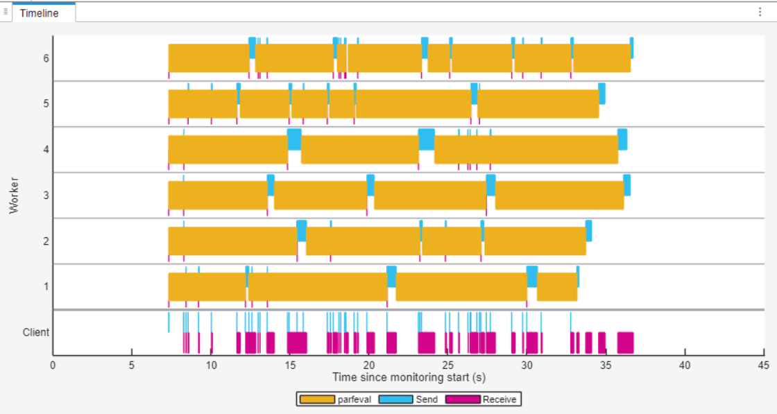
After the section code is complete, in the Monitoring section of the Pool Dashboard, select Stop.
The Timeline graph represents the time workers spend running parfeval computations in yellow. In the Timeline graph, you can observe that each worker completes multiple parfeval computations. Some workers remain idle for one to two seconds between parfeval computations while they transfer results data back to the client. However, the workers are idle for less time compared to the first parfor-loop.
Clean Up
Delete the image files after use.
Define Helper Functions
The fftImage function computes the FFT of an image and stores the results in a structure.
function output = fftImage(filename) % Read the image img = imread(fullfile("images",filename));
% Perform FFT imgFFT = fft2(double(img));
% Store the magnitude spectrum scanNum = "scan" + extract(filename,digitsPattern); output.scanNumber = scanNum; output.spectra = abs(fftshift(imgFFT)); end
The createFiles function generates images to process in the example and saves the images to the images folder.
function createFiles % Create folder to save images outputDir = "images"; if exist(outputDir,"dir") mkdir(outputDir); end
% Define clusters of image sizes sizes = [50 60 74 60 150 348 400 420 448 160 174 250 260 274]; fileSizes = repmat(sizes,1,4);
% Function to generate and save random images generateImages = @(fileSizes,outputDir,prefix) arrayfun(@(n) ... imwrite(repmat(peaks(20),[fileSizes(n)/2 fileSizes(n)]), ... fullfile(outputDir,sprintf("%s_image_%02d.jpg",prefix,n))),1:numel(fileSizes));
% Generate small, medium, and large images generateImages(fileSizes,outputDir,"scan");
fprintf("%d images generated.",numel(fileSizes)); end
The barSubranges function plots the size of the files in each subrange group in a bar chart.
function barSubranges(groupedImageFiles,subranges) % Initialize variables lastIdx = 0; bytes = [groupedImageFiles.bytes]; cumulativeSums = cumsum(subranges);
% Prepare data for the stacked bar chart stackedData = zeros(numel(subranges),max(subranges)); for idx = 1:numel(subranges) firstIdx = lastIdx + 1; lastIdx = cumulativeSums(idx); groupBytes = bytes(firstIdx:lastIdx); stackedData(idx,1:numel(groupBytes)) = groupBytes; end
% Plot the stacked bar chart figure; bar(stackedData,"stacked"); xlabel("Group Index"); ylabel("File Size (Bytes)"); title("File Sizes in Each Group"); legendStr = arrayfun(@(x) sprintf('File %d',x),1:size(stackedData,2),UniformOutput=false); legend(legendStr,Location="northeastoutside"); grid on; end