Programmatically Collect Pool Monitoring Data - MATLAB & Simulink (original) (raw)
Main Content
Pool monitoring data helps you understand how pool workers execute parallel constructs like parfor, parfeval, andspmd on parallel pools. Monitoring data includes information about how workers execute your parallel code and the data transfers involved. This information helps you identify bottlenecks, balance workloads, ensure efficient resource utilization, and optimize the performance of your parallel code.
You can collect pool activity monitoring data programmatically using anActivityMonitor object or interactively with the Pool Dashboard. For most workflows, use the Pool Dashboard to interactively collect and view monitoring data. However, if you need to collect monitoring data to review later or for code that runs on a batch parallel pool, use anActivityMonitor object.
Collect Monitoring Data on Interactive Parallel Pool
This example shows how to use an ActivityMonitor object to collect monitoring data on an interactive parallel pool.
Create a parallel pool with three workers.
nWorkers = 3; pool = parpool(nWorkers);
Starting parallel pool (parpool) using the 'Processes' profile ... Connected to parallel pool with 3 workers.
Collect and Analyze Monitoring Data
Create an ActivityMonitor object to start collecting pool monitoring data.
monitor = parallel.pool.ActivityMonitor;
Run your parallel code. For the purposes of this example, use a simple parfor-loop that iterates over a series of values.
values = [5 12 13 1 12 5]; parfor (idx = 1:numel(values),3) u = rand(values(idx)*3e4,1); out(idx) = max(conv(u,u)); end
After the code completes, stop collecting monitoring data and retrieve the pool monitoring results collected during the parfor execution.
monitoringResults = stop(monitor);
Visualize the monitoring results in the Pool Dashboard. The parpoolDashboard function opens the Pool Dashboard and displays the monitoring results in the ActivityMonitorResults object, monitoringResults.
parpoolDashboard(monitoringResults)
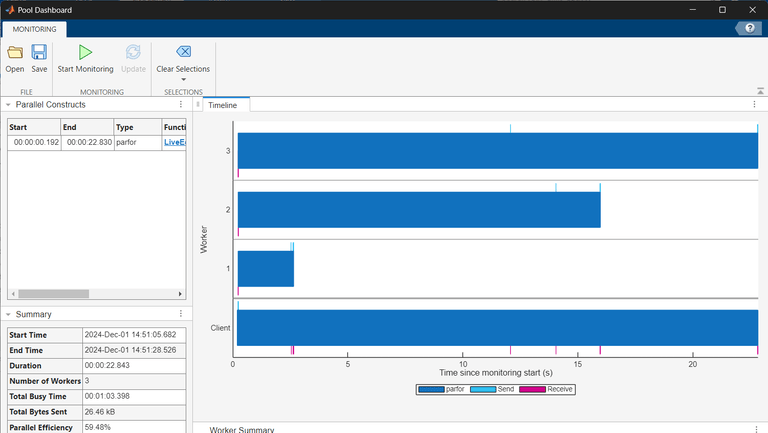
Generally, comparing the execution times of the workers can help you identify the bottlenecks in your code. The Timeline graph visually represents the time workers and the client spend executing the parfor-loop and transferring data. Dark blue indicates time spent running the parfor-loop, light blue represents time spent sending data, and magenta represents time spent receiving data.
You can observe that some workers take significantly longer to complete their iterations compared to other workers, which results in workers remaining idle for most of the parfor execution time. This observation suggests that the load is not distributed evenly across the workers.
Improve Parallel Code
If you know the workload of each iteration in your parfor-loop, then you can use parforOptions to control the partitioning of iterations into subranges for the workers. For more information, see parforOptions.
In this example, the greater the value in values, the more computationally intensive the iteration. Each consecutive pair of values in values balances low and high computational intensity. To distribute the workload better, create a set of parfor options to divide the parfor iterations into subranges of size 2.
opts = parforOptions(pool,RangePartitionMethod="fixed",SubrangeSize=2);
Create an ActivityMonitor object to start collecting pool monitoring data.
monitor = parallel.pool.ActivityMonitor;
Run the same code as before. To use the parfor options, pass them to the second input argument of parfor.
parfor (idx = 1:numel(values),opts) u = rand(values(idx)*3e4,1); out(idx) = max(conv(u,u)); end
Retrieve the monitoring results and visualize the results in the Pool Dashboard.
monitoringResults = stop(monitor); parpoolDashboard(monitoringResults)
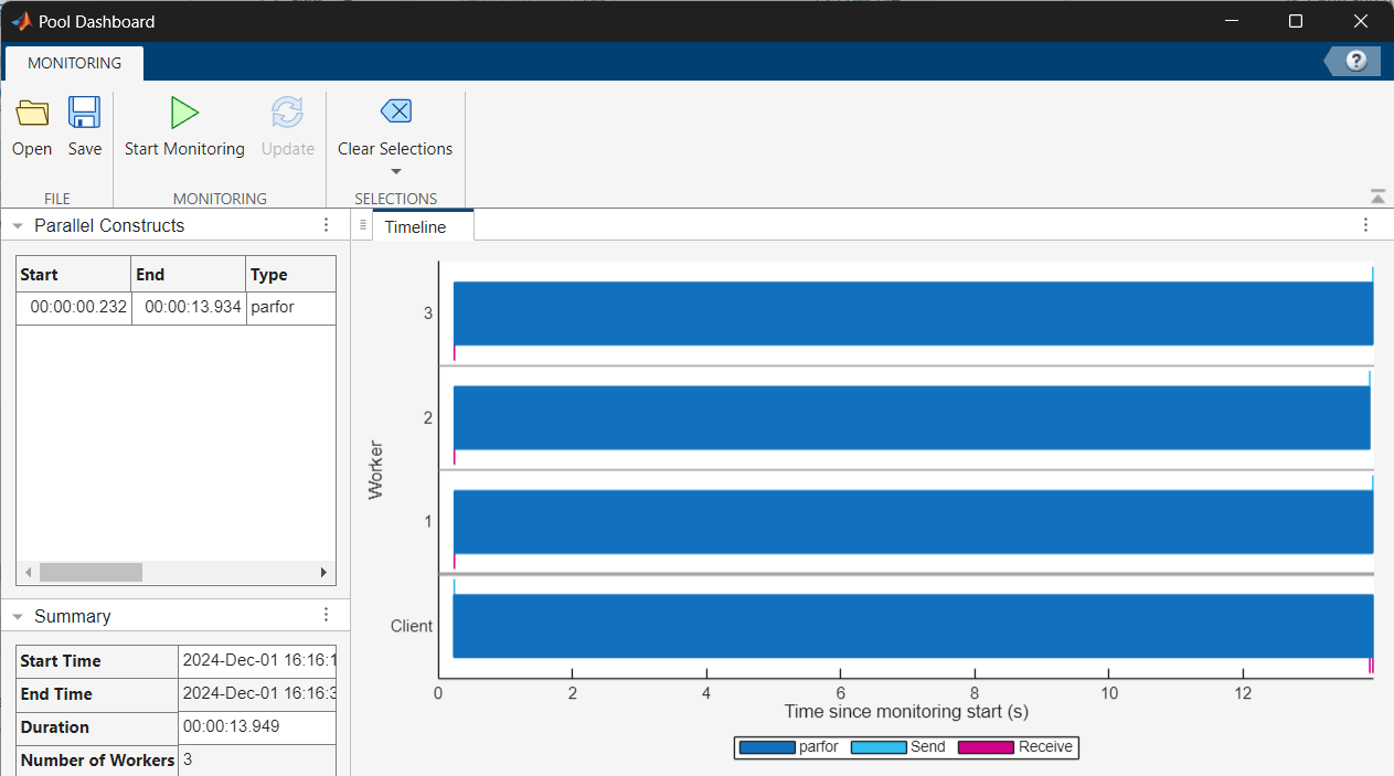
In the Timeline graph, compare the execution times of the workers. Observe that in the second parfor-loop, each worker takes a similar amount of time to execute their parfor iterations and there are no idle workers. The workload is now better distributed.
Collect Monitoring Data on Batch Parallel Pool
This example shows how to use an ActivityMonitor object to collect monitoring data on a parallel pool of a batch job.
Define a function that runs simulations of different dollar auction models using the parfeval function. The function creates an ActivityMonitor object to collect monitoring data, submits and waits for the parfeval computations, and retrieves the pool monitoring results.
function monitoringResults = runDollarAuctionModels % Define simulation parameters params.nPlayers = 20; params.incr = 0.05; params.dropoutRate = 0.01; params.nTrials = 1000; params.coalitionProbability = 0.5; params.riskRange = [0.5 2];
% Define a list of model functions to run modelFunctions = {@mcDollarAuction,@mcCollabDollarAuction,@mcRiskAverseDollarAuction}; numModels = length(modelFunctions);
% Create an ActivityMonitor object to collect monitoring data monitor = parallel.pool.ActivityMonitor;
% Use parfeval to simulate each model in parallel f(1:numModels) = parallel.FevalFuture; for m = 1:numModels f(m) = parfeval(modelFunctions{m},1,params); end wait(f);
% Stop the activity monitor and retrieve the results collected monitoringResults = stop(monitor); end
Run the runDollarAuctionModels function as a batch pool job and wait for the batch job to complete.
job = batch(@runDollarAuctionModels,1,Pool=4,CaptureDiary=false); wait(job);
Fetch the monitoring results from the completed batch job.
out = fetchOutputs(job); monitoringResults = out{1};
Visualize the monitoring results in the Pool Dashboard.
parpoolDashboard(monitoringResults)
Explore Pool Monitoring Data
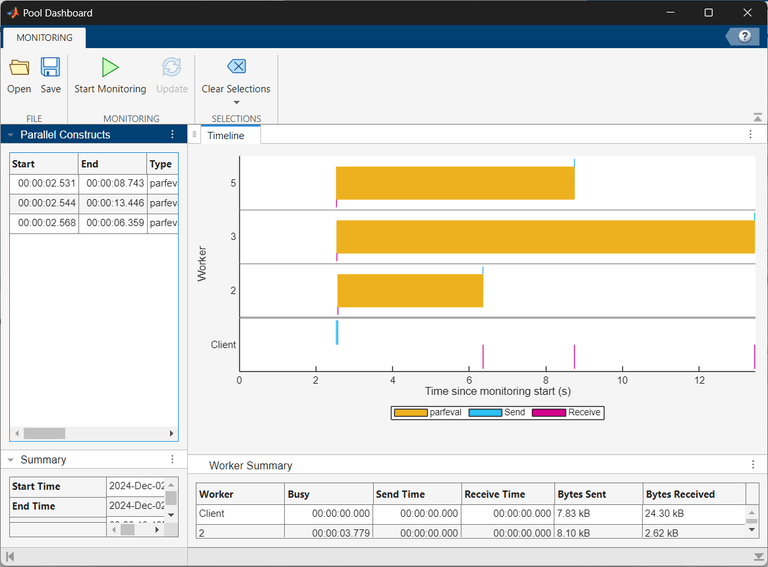
In the Pool Dashboard, the Timeline graph represents the time workers spend running the parallel code and transferring data. Yellow indicates time spent running the parfeval computations, light blue represents time spent sending data, and magenta represents time spent receiving data. Observing the Timeline graph, you can see that one parfeval bar is longer than the other bars. To view information specific to that parfeval computation, click the bar.
The Timeline graph and Parallel Constructs, Summary and Worker Summary tables now display information specific to the selected parfeval computation. You can identify which function the selected parfeval computation was running in the Parallel Constructs table, under the Details column.
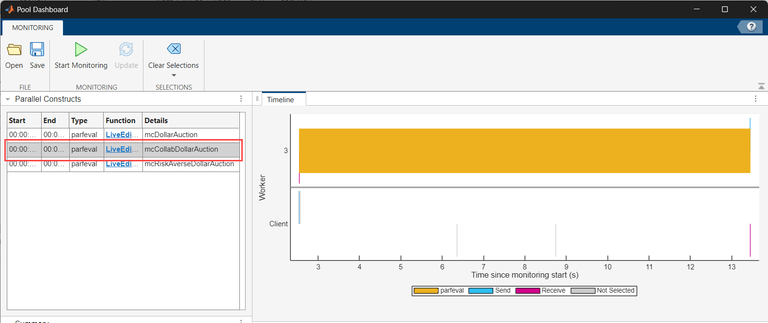
To clear the information for the currently selected parfeval computation and view activity data for all the workers again, in the Selections section of the Pool Dashboard, select Clear Selections.
See Also
Functions
- parfor | parfeval | stop | parforOptions