Comparing Performance - MATLAB & Simulink (original) (raw)
When simulation execution time exceeds the time required for code generation, accelerator and rapid accelerator simulation modes give speed improvement compared to normal mode. Accelerator and rapid accelerator modes generally perform better than normal mode when simulation execution times are several minutes or more. However, models with a significant number of Stateflow® or MATLAB Function blocks might show only a small speed improvement over normal mode because these blocks also simulate through code generation in normal mode.
Including tunable parameters in your model can also increase the simulation time.
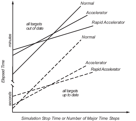
The figure shows the relative performance of normal mode, accelerator mode, and rapid accelerator mode simulations in general terms for a hypothetical model.
Performance When Target Must Be Rebuilt
The solid lines, labeled all targets out of date, in the figure show performance when the target code must be rebuilt. For this hypothetical model, the time scale is on the order of minutes. However, the time scale could be longer for more complex models.
Compiling a model in normal mode generally requires less time than building the accelerator target or the rapid accelerator executable. For small simulation stop times, normal mode results in quicker overall simulations compared to the accelerator and rapid accelerator modes.
The crossover point where accelerator mode or rapid accelerator mode results in faster overall simulation depends on the complexity and content of your model. For example, models that contain large numbers of blocks that use interpreted code might not run much faster in accelerator mode than they would in normal mode unless the simulation stop time is very large. For more information, see Select Blocks for Accelerator Mode. Similarly, models with a large number of Stateflow charts or MATLAB Function blocks might not show much speed improvement over normal mode unless the simulation stop time is large. You can speed up the simulation of models with Stateflow or MATLAB Function blocks through code generation.
The figure represents a model with a large number of Stateflow charts or MATLAB Function blocks. The curve labeled Normal would have a much smaller initial elapsed time than shown if the model did not contain these blocks.
Performance When Targets Are Up to Date
The dashed lines, labeled all targets up to date, in the figure show that the time to determine whether the accelerator target or the rapid accelerator executable is up to date is significantly smaller than the time required to generate code, which is represented by the solid lines, labeled all targets out of date. You can take advantage of this characteristic when you want to test various design tradeoffs.
For instance, you can generate the accelerator mode target once and use it to simulate your model with a series of gain settings. This method is especially efficient for the accelerator or rapid accelerator modes because this type of change does not result in the target code being regenerated. The target code is generated the first time the model runs, but on subsequent runs, the software spends only the time necessary to verify that the target is up to date. This process is much faster than generating code, so subsequent runs can be significantly faster than the initial run.
Because checking the targets is quicker than code generation, the crossover point is smaller when the target is up to date than when code must be generated. Subsequent runs of your model might simulate faster in accelerator or rapid accelerator mode when compared to normal mode, even for small stop times.
Analyze Performance of Simulation Modes
This example compares the performance of normal and rapid accelerator mode simulations for the model sldemo_fuelsys by running three simulations:
- The first simulation uses normal mode.
- The second simulation uses rapid accelerator mode and builds the rapid accelerator target.
- The third simulation uses rapid accelerator mode and does not build the rapid accelerator target.
To analyze the performance of each simulation, inspect the timing information returned with the simulation metadata. Simulation metadata is returned as a Simulink.SimulationMetadata object in the SimulationMetadata property of the Simulink.SimulationOutput object. The TimingInfo property of the Simulink.SimulationMetadata object provides the total simulation time as well as a breakdown of the time spent in each phase of the simulation.
Open the model.
To configure the baseline normal mode simulation, create a Simulink.SimulationInput object. The SimulationInput object stores parameter values to use in the simulation. The parameter values on the object are applied for the simulation and reverted at the end of simulation so that the model remains unchanged.
simin = Simulink.SimulationInput(mdl);
Set the stop time to 10000. Set the simulation mode to Normal.
simin = setModelParameter(simin,"StopTime","10000"); simin = setModelParameter(simin,"SimulationMode","normal");
To capture baseline timing information, simulate the model.
The simulation returns results as a single Simulink.SimulationOutput object. The SimulationMetadata property contains the simulation metadata, stored as a Simulink.SimulationMetadata object.
Use dot notation to store the contents of the TimingInfo property in a variable named normalMode.
normalMode = simOut.SimulationMetadata.TimingInfo;
From the timing information, extract the initialization time, execution time, and total elapsed time for the simulation.
normalInit = normalMode.InitializationElapsedWallTime; normalExec = normalMode.ExecutionElapsedWallTime; normalTotal = normalMode.TotalElapsedWallTime;
Simulate the model again using rapid accelerator mode. The first time you simulate a model in rapid accelerator mode, the rapid accelerator target builds during the initialization phase.
simin = setModelParameter(simin,"SimulationMode","rapid"); simOut = sim(simin);
Searching for referenced models in model 'sldemo_fuelsys'.
Total of 1 models to build.
Building the rapid accelerator target for model: sldemo_fuelsys
Successfully built the rapid accelerator target for model: sldemo_fuelsys
Get the timing information for the first rapid accelerator simulation. Then, extract the initialization time, execution time, and total elapsed time for the simulation.
rapidAccel = simOut.SimulationMetadata.TimingInfo; rapidBuildInit = rapidAccel.InitializationElapsedWallTime; rapidBuildExec = rapidAccel.ExecutionElapsedWallTime; rapidBuildTotal = rapidAccel.TotalElapsedWallTime;
Simulate again to see the benefit of rapid accelerator mode for a simulation that does not build the rapid accelerator target.
Searching for referenced models in model 'sldemo_fuelsys'.
Total of 1 models to build.
Get the timing information for the rapid accelerator simulation that ran without building the target. Then, extract the initialization time, the execution time, and the total elapsed time for the simulation.
rapidAccelNoRebuild = simOut.SimulationMetadata.TimingInfo; rapidInit = rapidAccelNoRebuild.InitializationElapsedWallTime; rapidExec = rapidAccelNoRebuild.ExecutionElapsedWallTime; rapidTotal = rapidAccelNoRebuild.TotalElapsedWallTime;
Build a table to compare the timing for each simulation.
Normal = [normalInit;normalExec;normalTotal]; RapidBuild = [rapidBuildInit;rapidBuildExec;rapidBuildTotal]; RapidNoBuild = [rapidInit;rapidExec;rapidTotal];
names = ["Initialization Time"; "Execution Time"; "Total Simulation Time"];
timingTable = table(Normal,RapidBuild,RapidNoBuild,RowNames=names);
In the first rapid accelerator simulation, the initialization time increases because the rapid accelerator target builds during the initialization phase. For this model and simulation duration, using rapid accelerator mode reduces the execution time so much that the first rapid accelerator simulation is still faster than using normal mode.
timingTable=3×3 table Normal RapidBuild RapidNoBuild ______ __________ ____________
Initialization Time      9.1109      24.371         2.1894
Execution Time           121.25      52.275         40.829
Total Simulation Time     130.4      76.751         43.115
See Also
Simulink.SimulationInput | Simulink.SimulationOutput