Indexing and selecting data — pandas 3.0.0.dev0+2095.g2e141aaf99 documentation (original) (raw)

The axis labeling information in pandas objects serves many purposes:

• Identifies data (i.e. provides metadata) using known indicators, important for analysis, visualization, and interactive console display.
• Enables automatic and explicit data alignment.
• Allows intuitive getting and setting of subsets of the data set.

In this section, we will focus on the final point: namely, how to slice, dice, and generally get and set subsets of pandas objects. The primary focus will be on Series and DataFrame as they have received more development attention in this area.

Note

The Python and NumPy indexing operators [] and attribute operator .provide quick and easy access to pandas data structures across a wide range of use cases. This makes interactive work intuitive, as there’s little new to learn if you already know how to deal with Python dictionaries and NumPy arrays. However, since the type of the data to be accessed isn’t known in advance, directly using standard operators has some optimization limits. For production code, we recommended that you take advantage of the optimized pandas data access methods exposed in this chapter.

See the MultiIndex / Advanced Indexing for MultiIndex and more advanced indexing documentation.

See the cookbook for some advanced strategies.

Different choices for indexing#

Object selection has had a number of user-requested additions in order to support more explicit location based indexing. pandas now supports three types of multi-axis indexing.

• .loc is primarily label based, but may also be used with a boolean array. .loc will raise KeyError when the items are not found. Allowed inputs are:

  • A single label, e.g. 5 or 'a' (Note that 5 is interpreted as a_label_ of the index. This use is not an integer position along the index.).
  • A list or array of labels ['a', 'b', 'c'].
  • A slice object with labels 'a':'f' (Note that contrary to usual Python slices, both the start and the stop are included, when present in the index! See Slicing with labelsand Endpoints are inclusive.)
  • A boolean array (any NA values will be treated as False).
  • A callable function with one argument (the calling Series or DataFrame) and that returns valid output for indexing (one of the above).
  • A tuple of row (and column) indices whose elements are one of the above inputs.
    See more at Selection by Label.

• .iloc is primarily integer position based (from 0 tolength-1 of the axis), but may also be used with a boolean array. .iloc will raise IndexError if a requested indexer is out-of-bounds, except slice indexers which allow out-of-bounds indexing. (this conforms with Python/NumPy _slice_semantics). Allowed inputs are:

  • An integer e.g. 5.
  • A list or array of integers [4, 3, 0].
  • A slice object with ints 1:7.
  • A boolean array (any NA values will be treated as False).
  • A callable function with one argument (the calling Series or DataFrame) and that returns valid output for indexing (one of the above).
  • A tuple of row (and column) indices whose elements are one of the above inputs.
    See more at Selection by Position,Advanced Indexing and Advanced Hierarchical.

• .loc, .iloc, and also [] indexing can accept a callable as indexer. See more at Selection By Callable.
  Note
  Destructuring tuple keys into row (and column) indexes occurs_before_ callables are applied, so you cannot return a tuple from a callable to index both rows and columns.

Getting values from an object with multi-axes selection uses the following notation (using .loc as an example, but the following applies to .iloc as well). Any of the axes accessors may be the null slice :. Axes left out of the specification are assumed to be :, e.g. p.loc['a'] is equivalent top.loc['a', :].

In [1]: ser = pd.Series(range(5), index=list("abcde"))

In [2]: ser.loc[["a", "c", "e"]] Out[2]: a 0 c 2 e 4 dtype: int64

In [3]: df = pd.DataFrame(np.arange(25).reshape(5, 5), index=list("abcde"), columns=list("abcde"))

In [4]: df.loc[["a", "c", "e"], ["b", "d"]] Out[4]: b d a 1 3 c 11 13 e 21 23

Basics#

As mentioned when introducing the data structures in the last section, the primary function of indexing with [] (a.k.a. __getitem__for those familiar with implementing class behavior in Python) is selecting out lower-dimensional slices. The following table shows return type values when indexing pandas objects with []:

Here we construct a simple time series data set to use for illustrating the indexing functionality:

In [5]: dates = pd.date_range('1/1/2000', periods=8)

In [6]: df = pd.DataFrame(np.random.randn(8, 4), ...: index=dates, columns=['A', 'B', 'C', 'D']) ...:

In [7]: df Out[7]: A B C D 2000-01-01 0.469112 -0.282863 -1.509059 -1.135632 2000-01-02 1.212112 -0.173215 0.119209 -1.044236 2000-01-03 -0.861849 -2.104569 -0.494929 1.071804 2000-01-04 0.721555 -0.706771 -1.039575 0.271860 2000-01-05 -0.424972 0.567020 0.276232 -1.087401 2000-01-06 -0.673690 0.113648 -1.478427 0.524988 2000-01-07 0.404705 0.577046 -1.715002 -1.039268 2000-01-08 -0.370647 -1.157892 -1.344312 0.844885

Note

None of the indexing functionality is time series specific unless specifically stated.

Thus, as per above, we have the most basic indexing using []:

In [8]: s = df['A']

In [9]: s[dates[5]] Out[9]: np.float64(-0.6736897080883706)

You can pass a list of columns to [] to select columns in that order. If a column is not contained in the DataFrame, an exception will be raised. Multiple columns can also be set in this manner:

In [10]: df Out[10]: A B C D 2000-01-01 0.469112 -0.282863 -1.509059 -1.135632 2000-01-02 1.212112 -0.173215 0.119209 -1.044236 2000-01-03 -0.861849 -2.104569 -0.494929 1.071804 2000-01-04 0.721555 -0.706771 -1.039575 0.271860 2000-01-05 -0.424972 0.567020 0.276232 -1.087401 2000-01-06 -0.673690 0.113648 -1.478427 0.524988 2000-01-07 0.404705 0.577046 -1.715002 -1.039268 2000-01-08 -0.370647 -1.157892 -1.344312 0.844885

In [11]: df[['B', 'A']] = df[['A', 'B']]

In [12]: df Out[12]: A B C D 2000-01-01 -0.282863 0.469112 -1.509059 -1.135632 2000-01-02 -0.173215 1.212112 0.119209 -1.044236 2000-01-03 -2.104569 -0.861849 -0.494929 1.071804 2000-01-04 -0.706771 0.721555 -1.039575 0.271860 2000-01-05 0.567020 -0.424972 0.276232 -1.087401 2000-01-06 0.113648 -0.673690 -1.478427 0.524988 2000-01-07 0.577046 0.404705 -1.715002 -1.039268 2000-01-08 -1.157892 -0.370647 -1.344312 0.844885

You may find this useful for applying a transform (in-place) to a subset of the columns.

Warning

pandas aligns all AXES when setting Series and DataFrame from .loc.

This will not modify df because the column alignment is before value assignment.

In [13]: df[['A', 'B']] Out[13]: A B 2000-01-01 -0.282863 0.469112 2000-01-02 -0.173215 1.212112 2000-01-03 -2.104569 -0.861849 2000-01-04 -0.706771 0.721555 2000-01-05 0.567020 -0.424972 2000-01-06 0.113648 -0.673690 2000-01-07 0.577046 0.404705 2000-01-08 -1.157892 -0.370647

In [14]: df.loc[:, ['B', 'A']] = df[['A', 'B']]

In [15]: df[['A', 'B']] Out[15]: A B 2000-01-01 -0.282863 0.469112 2000-01-02 -0.173215 1.212112 2000-01-03 -2.104569 -0.861849 2000-01-04 -0.706771 0.721555 2000-01-05 0.567020 -0.424972 2000-01-06 0.113648 -0.673690 2000-01-07 0.577046 0.404705 2000-01-08 -1.157892 -0.370647

The correct way to swap column values is by using raw values:

In [16]: df.loc[:, ['B', 'A']] = df[['A', 'B']].to_numpy()

In [17]: df[['A', 'B']] Out[17]: A B 2000-01-01 0.469112 -0.282863 2000-01-02 1.212112 -0.173215 2000-01-03 -0.861849 -2.104569 2000-01-04 0.721555 -0.706771 2000-01-05 -0.424972 0.567020 2000-01-06 -0.673690 0.113648 2000-01-07 0.404705 0.577046 2000-01-08 -0.370647 -1.157892

However, pandas does not align AXES when setting Series and DataFrame from .ilocbecause .iloc operates by position.

This will modify df because the column alignment is not done before value assignment.

In [18]: df[['A', 'B']] Out[18]: A B 2000-01-01 0.469112 -0.282863 2000-01-02 1.212112 -0.173215 2000-01-03 -0.861849 -2.104569 2000-01-04 0.721555 -0.706771 2000-01-05 -0.424972 0.567020 2000-01-06 -0.673690 0.113648 2000-01-07 0.404705 0.577046 2000-01-08 -0.370647 -1.157892

In [19]: df.iloc[:, [1, 0]] = df[['A', 'B']]

In [20]: df[['A','B']] Out[20]: A B 2000-01-01 -0.282863 0.469112 2000-01-02 -0.173215 1.212112 2000-01-03 -2.104569 -0.861849 2000-01-04 -0.706771 0.721555 2000-01-05 0.567020 -0.424972 2000-01-06 0.113648 -0.673690 2000-01-07 0.577046 0.404705 2000-01-08 -1.157892 -0.370647

Attribute access#

You may access an index on a Series or column on a DataFrame directly as an attribute:

In [21]: sa = pd.Series([1, 2, 3], index=list('abc'))

In [22]: dfa = df.copy()

In [23]: sa.b Out[23]: np.int64(2)

In [24]: dfa.A Out[24]: 2000-01-01 -0.282863 2000-01-02 -0.173215 2000-01-03 -2.104569 2000-01-04 -0.706771 2000-01-05 0.567020 2000-01-06 0.113648 2000-01-07 0.577046 2000-01-08 -1.157892 Freq: D, Name: A, dtype: float64

In [25]: sa.a = 5

In [26]: sa Out[26]: a 5 b 2 c 3 dtype: int64

In [27]: dfa.A = list(range(len(dfa.index))) # ok if A already exists

In [28]: dfa Out[28]: A B C D 2000-01-01 0 0.469112 -1.509059 -1.135632 2000-01-02 1 1.212112 0.119209 -1.044236 2000-01-03 2 -0.861849 -0.494929 1.071804 2000-01-04 3 0.721555 -1.039575 0.271860 2000-01-05 4 -0.424972 0.276232 -1.087401 2000-01-06 5 -0.673690 -1.478427 0.524988 2000-01-07 6 0.404705 -1.715002 -1.039268 2000-01-08 7 -0.370647 -1.344312 0.844885

In [29]: dfa['A'] = list(range(len(dfa.index))) # use this form to create a new column

In [30]: dfa Out[30]: A B C D 2000-01-01 0 0.469112 -1.509059 -1.135632 2000-01-02 1 1.212112 0.119209 -1.044236 2000-01-03 2 -0.861849 -0.494929 1.071804 2000-01-04 3 0.721555 -1.039575 0.271860 2000-01-05 4 -0.424972 0.276232 -1.087401 2000-01-06 5 -0.673690 -1.478427 0.524988 2000-01-07 6 0.404705 -1.715002 -1.039268 2000-01-08 7 -0.370647 -1.344312 0.844885

Warning

• You can use this access only if the index element is a valid Python identifier, e.g. s.1 is not allowed. See here for an explanation of valid identifiers.
• The attribute will not be available if it conflicts with an existing method name, e.g. s.min is not allowed, but s['min'] is possible.
• Similarly, the attribute will not be available if it conflicts with any of the following list: index,major_axis, minor_axis, items.
• In any of these cases, standard indexing will still work, e.g. s['1'], s['min'], and s['index'] will access the corresponding element or column.

If you are using the IPython environment, you may also use tab-completion to see these accessible attributes.

You can also assign a dict to a row of a DataFrame:

In [31]: x = pd.DataFrame({'x': [1, 2, 3], 'y': [3, 4, 5]})

In [32]: x.iloc[1] = {'x': 9, 'y': 99}

In [33]: x Out[33]: x y 0 1 3 1 9 99 2 3 5

You can use attribute access to modify an existing element of a Series or column of a DataFrame, but be careful; if you try to use attribute access to create a new column, it creates a new attribute rather than a new column and will this raise a UserWarning:

In [34]: df_new = pd.DataFrame({'one': [1., 2., 3.]})

In [35]: df_new.two = [4, 5, 6]

In [36]: df_new Out[36]: one 0 1.0 1 2.0 2 3.0

Slicing ranges#

The most robust and consistent way of slicing ranges along arbitrary axes is described in the Selection by Position section detailing the .iloc method. For now, we explain the semantics of slicing using the [] operator.

Note

When the Series has float indices, slicing will select by position.

With Series, the syntax works exactly as with an ndarray, returning a slice of the values and the corresponding labels:

In [37]: s[:5] Out[37]: 2000-01-01 0.469112 2000-01-02 1.212112 2000-01-03 -0.861849 2000-01-04 0.721555 2000-01-05 -0.424972 Freq: D, Name: A, dtype: float64

In [38]: s[::2] Out[38]: 2000-01-01 0.469112 2000-01-03 -0.861849 2000-01-05 -0.424972 2000-01-07 0.404705 Freq: 2D, Name: A, dtype: float64

In [39]: s[::-1] Out[39]: 2000-01-08 -0.370647 2000-01-07 0.404705 2000-01-06 -0.673690 2000-01-05 -0.424972 2000-01-04 0.721555 2000-01-03 -0.861849 2000-01-02 1.212112 2000-01-01 0.469112 Freq: -1D, Name: A, dtype: float64

Note that setting works as well:

In [40]: s2 = s.copy()

In [41]: s2[:5] = 0

In [42]: s2 Out[42]: 2000-01-01 0.000000 2000-01-02 0.000000 2000-01-03 0.000000 2000-01-04 0.000000 2000-01-05 0.000000 2000-01-06 -0.673690 2000-01-07 0.404705 2000-01-08 -0.370647 Freq: D, Name: A, dtype: float64

With DataFrame, slicing inside of [] slices the rows. This is provided largely as a convenience since it is such a common operation.

In [43]: df[:3] Out[43]: A B C D 2000-01-01 -0.282863 0.469112 -1.509059 -1.135632 2000-01-02 -0.173215 1.212112 0.119209 -1.044236 2000-01-03 -2.104569 -0.861849 -0.494929 1.071804

In [44]: df[::-1] Out[44]: A B C D 2000-01-08 -1.157892 -0.370647 -1.344312 0.844885 2000-01-07 0.577046 0.404705 -1.715002 -1.039268 2000-01-06 0.113648 -0.673690 -1.478427 0.524988 2000-01-05 0.567020 -0.424972 0.276232 -1.087401 2000-01-04 -0.706771 0.721555 -1.039575 0.271860 2000-01-03 -2.104569 -0.861849 -0.494929 1.071804 2000-01-02 -0.173215 1.212112 0.119209 -1.044236 2000-01-01 -0.282863 0.469112 -1.509059 -1.135632

Selection by label#

Warning

.loc is strict when you present slicers that are not compatible (or convertible) with the index type. For example using integers in a DatetimeIndex. These will raise a TypeError.

In [45]: dfl = pd.DataFrame(np.random.randn(5, 4), ....: columns=list('ABCD'), ....: index=pd.date_range('20130101', periods=5)) ....:

In [46]: dfl Out[46]: A B C D 2013-01-01 1.075770 -0.109050 1.643563 -1.469388 2013-01-02 0.357021 -0.674600 -1.776904 -0.968914 2013-01-03 -1.294524 0.413738 0.276662 -0.472035 2013-01-04 -0.013960 -0.362543 -0.006154 -0.923061 2013-01-05 0.895717 0.805244 -1.206412 2.565646

In [47]: dfl.loc[2:3]

TypeError Traceback (most recent call last) Cell In[47], line 1 ----> 1 dfl.loc[2:3]

File ~/work/pandas/pandas/pandas/core/indexing.py:1196, in _LocationIndexer.getitem(self, key) 1194 maybe_callable = com.apply_if_callable(key, self.obj) 1195 maybe_callable = self._raise_callable_usage(key, maybe_callable) -> 1196 return self._getitem_axis(maybe_callable, axis=axis)

File ~/work/pandas/pandas/pandas/core/indexing.py:1418, in _LocIndexer._getitem_axis(self, key, axis) 1416 if isinstance(key, slice): 1417 self._validate_key(key, axis) -> 1418 return self._get_slice_axis(key, axis=axis) 1419 elif com.is_bool_indexer(key): 1420 return self._getbool_axis(key, axis=axis)

File ~/work/pandas/pandas/pandas/core/indexing.py:1450, in _LocIndexer._get_slice_axis(self, slice_obj, axis) 1447 return obj.copy(deep=False) 1449 labels = obj._get_axis(axis) -> 1450 indexer = labels.slice_indexer(slice_obj.start, slice_obj.stop, slice_obj.step) 1452 if isinstance(indexer, slice): 1453 return self.obj._slice(indexer, axis=axis)

File ~/work/pandas/pandas/pandas/core/indexes/datetimes.py:673, in DatetimeIndex.slice_indexer(self, start, end, step) 665 # GH#33146 if start and end are combinations of str and None and Index is not 666 # monotonic, we can not use Index.slice_indexer because it does not honor the 667 # actual elements, is only searching for start and end 668 if ( 669 check_str_or_none(start) 670 or check_str_or_none(end) 671 or self.is_monotonic_increasing 672 ): --> 673 return Index.slice_indexer(self, start, end, step) 675 mask = np.array(True) 676 in_index = True

File ~/work/pandas/pandas/pandas/core/indexes/base.py:6562, in Index.slice_indexer(self, start, end, step) 6511 def slice_indexer( 6512 self, 6513 start: Hashable | None = None, 6514 end: Hashable | None = None, 6515 step: int | None = None, 6516 ) -> slice: 6517 """ 6518 Compute the slice indexer for input labels and step. 6519 (...) 6560 slice(1, 3, None) 6561 """ -> 6562 start_slice, end_slice = self.slice_locs(start, end, step=step) 6564 # return a slice 6565 if not is_scalar(start_slice):

File ~/work/pandas/pandas/pandas/core/indexes/base.py:6802, in Index.slice_locs(self, start, end, step) 6800 start_slice = None 6801 if start is not None: -> 6802 start_slice = self.get_slice_bound(start, "left") 6803 if start_slice is None: 6804 start_slice = 0

File ~/work/pandas/pandas/pandas/core/indexes/base.py:6706, in Index.get_slice_bound(self, label, side) 6702 original_label = label 6704 # For datetime indices label may be a string that has to be converted 6705 # to datetime boundary according to its resolution. -> 6706 label = self._maybe_cast_slice_bound(label, side) 6708 # we need to look up the label 6709 try:

File ~/work/pandas/pandas/pandas/core/indexes/datetimes.py:633, in DatetimeIndex._maybe_cast_slice_bound(self, label, side) 628 if isinstance(label, dt.date) and not isinstance(label, dt.datetime): 629 # Pandas supports slicing with dates, treated as datetimes at midnight. 630 # https://github.com/pandas-dev/pandas/issues/31501 631 label = Timestamp(label).to_pydatetime() --> 633 label = super()._maybe_cast_slice_bound(label, side) 634 self._data._assert_tzawareness_compat(label) 635 return Timestamp(label)

File ~/work/pandas/pandas/pandas/core/indexes/datetimelike.py:369, in DatetimeIndexOpsMixin._maybe_cast_slice_bound(self, label, side) 367 return lower if side == "left" else upper 368 elif not isinstance(label, self._data._recognized_scalars): --> 369 self._raise_invalid_indexer("slice", label) 371 return label

File ~/work/pandas/pandas/pandas/core/indexes/base.py:4072, in Index._raise_invalid_indexer(self, form, key, reraise) 4070 if reraise is not lib.no_default: 4071 raise TypeError(msg) from reraise -> 4072 raise TypeError(msg)

TypeError: cannot do slice indexing on DatetimeIndex with these indexers [2] of type int

String likes in slicing can be convertible to the type of the index and lead to natural slicing.

In [48]: dfl.loc['20130102':'20130104'] Out[48]: A B C D 2013-01-02 0.357021 -0.674600 -1.776904 -0.968914 2013-01-03 -1.294524 0.413738 0.276662 -0.472035 2013-01-04 -0.013960 -0.362543 -0.006154 -0.923061

pandas provides a suite of methods in order to have purely label based indexing. This is a strict inclusion based protocol. Every label asked for must be in the index, or a KeyError will be raised. When slicing, both the start bound AND the stop bound are included, if present in the index. Integers are valid labels, but they refer to the label and not the position.

The .loc attribute is the primary access method. The following are valid inputs:

• A single label, e.g. 5 or 'a' (Note that 5 is interpreted as a label of the index. This use is not an integer position along the index.).
• A list or array of labels ['a', 'b', 'c'].
• A slice object with labels 'a':'f' (Note that contrary to usual Python slices, both the start and the stop are included, when present in the index! See Slicing with labels.
• A boolean array.
• A callable, see Selection By Callable.

In [49]: s1 = pd.Series(np.random.randn(6), index=list('abcdef'))

In [50]: s1 Out[50]: a 1.431256 b 1.340309 c -1.170299 d -0.226169 e 0.410835 f 0.813850 dtype: float64

In [51]: s1.loc['c':] Out[51]: c -1.170299 d -0.226169 e 0.410835 f 0.813850 dtype: float64

In [52]: s1.loc['b'] Out[52]: np.float64(1.3403088497993827)

Note that setting works as well:

In [53]: s1.loc['c':] = 0

In [54]: s1 Out[54]: a 1.431256 b 1.340309 c 0.000000 d 0.000000 e 0.000000 f 0.000000 dtype: float64

With a DataFrame:

In [55]: df1 = pd.DataFrame(np.random.randn(6, 4), ....: index=list('abcdef'), ....: columns=list('ABCD')) ....:

In [56]: df1 Out[56]: A B C D a 0.132003 -0.827317 -0.076467 -1.187678 b 1.130127 -1.436737 -1.413681 1.607920 c 1.024180 0.569605 0.875906 -2.211372 d 0.974466 -2.006747 -0.410001 -0.078638 e 0.545952 -1.219217 -1.226825 0.769804 f -1.281247 -0.727707 -0.121306 -0.097883

In [57]: df1.loc[['a', 'b', 'd'], :] Out[57]: A B C D a 0.132003 -0.827317 -0.076467 -1.187678 b 1.130127 -1.436737 -1.413681 1.607920 d 0.974466 -2.006747 -0.410001 -0.078638

Accessing via label slices:

In [58]: df1.loc['d':, 'A':'C'] Out[58]: A B C d 0.974466 -2.006747 -0.410001 e 0.545952 -1.219217 -1.226825 f -1.281247 -0.727707 -0.121306

For getting a cross section using a label (equivalent to df.xs('a')):

In [59]: df1.loc['a'] Out[59]: A 0.132003 B -0.827317 C -0.076467 D -1.187678 Name: a, dtype: float64

For getting values with a boolean array:

In [60]: df1.loc['a'] > 0 Out[60]: A True B False C False D False Name: a, dtype: bool

In [61]: df1.loc[:, df1.loc['a'] > 0] Out[61]: A a 0.132003 b 1.130127 c 1.024180 d 0.974466 e 0.545952 f -1.281247

NA values in a boolean array propagate as False:

In [62]: mask = pd.array([True, False, True, False, pd.NA, False], dtype="boolean")

In [63]: mask Out[63]: [True, False, True, False, , False] Length: 6, dtype: boolean

In [64]: df1[mask] Out[64]: A B C D a 0.132003 -0.827317 -0.076467 -1.187678 c 1.024180 0.569605 0.875906 -2.211372

For getting a value explicitly:

this is also equivalent to df1.at['a','A']

In [65]: df1.loc['a', 'A'] Out[65]: np.float64(0.13200317033032932)

Slicing with labels#

When using .loc with slices, if both the start and the stop labels are present in the index, then elements located between the two (including them) are returned:

In [66]: s = pd.Series(list('abcde'), index=[0, 3, 2, 5, 4])

In [67]: s.loc[3:5] Out[67]: 3 b 2 c 5 d dtype: object

If the index is sorted, and can be compared against start and stop labels, then slicing will still work as expected, by selecting labels which _rank_between the two:

In [68]: s.sort_index() Out[68]: 0 a 2 c 3 b 4 e 5 d dtype: object

In [69]: s.sort_index().loc[1:6] Out[69]: 2 c 3 b 4 e 5 d dtype: object

However, if at least one of the two is absent and the index is not sorted, an error will be raised (since doing otherwise would be computationally expensive, as well as potentially ambiguous for mixed type indexes). For instance, in the above example, s.loc[1:6] would raise KeyError.

For the rationale behind this behavior, seeEndpoints are inclusive.

In [70]: s = pd.Series(list('abcdef'), index=[0, 3, 2, 5, 4, 2])

In [71]: s.loc[3:5] Out[71]: 3 b 2 c 5 d dtype: object

Also, if the index has duplicate labels and either the start or the stop label is duplicated, an error will be raised. For instance, in the above example, s.loc[2:5] would raise a KeyError.

For more information about duplicate labels, seeDuplicate Labels.

Selection by position#

pandas provides a suite of methods in order to get purely integer based indexing. The semantics follow closely Python and NumPy slicing. These are 0-based indexing. When slicing, the start bound is included, while the upper bound is excluded. Trying to use a non-integer, even a valid label will raise an IndexError.

The .iloc attribute is the primary access method. The following are valid inputs:

• An integer e.g. 5.
• A list or array of integers [4, 3, 0].
• A slice object with ints 1:7.
• A boolean array.
• A callable, see Selection By Callable.
• A tuple of row (and column) indexes, whose elements are one of the above types.

In [72]: s1 = pd.Series(np.random.randn(5), index=list(range(0, 10, 2)))

In [73]: s1 Out[73]: 0 0.695775 2 0.341734 4 0.959726 6 -1.110336 8 -0.619976 dtype: float64

In [74]: s1.iloc[:3] Out[74]: 0 0.695775 2 0.341734 4 0.959726 dtype: float64

In [75]: s1.iloc[3] Out[75]: np.float64(-1.110336102891167)

Note that setting works as well:

In [76]: s1.iloc[:3] = 0

In [77]: s1 Out[77]: 0 0.000000 2 0.000000 4 0.000000 6 -1.110336 8 -0.619976 dtype: float64

With a DataFrame:

In [78]: df1 = pd.DataFrame(np.random.randn(6, 4), ....: index=list(range(0, 12, 2)), ....: columns=list(range(0, 8, 2))) ....:

In [79]: df1 Out[79]: 0 2 4 6 0 0.149748 -0.732339 0.687738 0.176444 2 0.403310 -0.154951 0.301624 -2.179861 4 -1.369849 -0.954208 1.462696 -1.743161 6 -0.826591 -0.345352 1.314232 0.690579 8 0.995761 2.396780 0.014871 3.357427 10 -0.317441 -1.236269 0.896171 -0.487602

Select via integer slicing:

In [80]: df1.iloc[:3] Out[80]: 0 2 4 6 0 0.149748 -0.732339 0.687738 0.176444 2 0.403310 -0.154951 0.301624 -2.179861 4 -1.369849 -0.954208 1.462696 -1.743161

In [81]: df1.iloc[1:5, 2:4] Out[81]: 4 6 2 0.301624 -2.179861 4 1.462696 -1.743161 6 1.314232 0.690579 8 0.014871 3.357427

Select via integer list:

In [82]: df1.iloc[[1, 3, 5], [1, 3]] Out[82]: 2 6 2 -0.154951 -2.179861 6 -0.345352 0.690579 10 -1.236269 -0.487602

In [83]: df1.iloc[1:3, :] Out[83]: 0 2 4 6 2 0.403310 -0.154951 0.301624 -2.179861 4 -1.369849 -0.954208 1.462696 -1.743161

In [84]: df1.iloc[:, 1:3] Out[84]: 2 4 0 -0.732339 0.687738 2 -0.154951 0.301624 4 -0.954208 1.462696 6 -0.345352 1.314232 8 2.396780 0.014871 10 -1.236269 0.896171

this is also equivalent to df1.iat[1,1]

In [85]: df1.iloc[1, 1] Out[85]: np.float64(-0.1549507744249032)

For getting a cross section using an integer position (equiv to df.xs(1)):

In [86]: df1.iloc[1] Out[86]: 0 0.403310 2 -0.154951 4 0.301624 6 -2.179861 Name: 2, dtype: float64

Out of range slice indexes are handled gracefully just as in Python/NumPy.

these are allowed in Python/NumPy.

In [87]: x = list('abcdef')

In [88]: x Out[88]: ['a', 'b', 'c', 'd', 'e', 'f']

In [89]: x[4:10] Out[89]: ['e', 'f']

In [90]: x[8:10] Out[90]: []

In [91]: s = pd.Series(x)

In [92]: s Out[92]: 0 a 1 b 2 c 3 d 4 e 5 f dtype: object

In [93]: s.iloc[4:10] Out[93]: 4 e 5 f dtype: object

In [94]: s.iloc[8:10] Out[94]: Series([], dtype: object)

Note that using slices that go out of bounds can result in an empty axis (e.g. an empty DataFrame being returned).

In [95]: dfl = pd.DataFrame(np.random.randn(5, 2), columns=list('AB'))

In [96]: dfl Out[96]: A B 0 -0.082240 -2.182937 1 0.380396 0.084844 2 0.432390 1.519970 3 -0.493662 0.600178 4 0.274230 0.132885

In [97]: dfl.iloc[:, 2:3] Out[97]: Empty DataFrame Columns: [] Index: [0, 1, 2, 3, 4]

In [98]: dfl.iloc[:, 1:3] Out[98]: B 0 -2.182937 1 0.084844 2 1.519970 3 0.600178 4 0.132885

In [99]: dfl.iloc[4:6] Out[99]: A B 4 0.27423 0.132885

A single indexer that is out of bounds will raise an IndexError. A list of indexers where any element is out of bounds will raise anIndexError.

In [100]: dfl.iloc[[4, 5, 6]]

IndexError Traceback (most recent call last) File ~/work/pandas/pandas/pandas/core/indexing.py:1716, in _iLocIndexer._get_list_axis(self, key, axis) 1715 try: -> 1716 return self.obj.take(key, axis=axis) 1717 except IndexError as err: 1718 # re-raise with different error message, e.g. test_getitem_ndarray_3d

File ~/work/pandas/pandas/pandas/core/generic.py:4045, in NDFrame.take(self, indices, axis, **kwargs) 4043 return self.copy(deep=False) -> 4045 new_data = self._mgr.take( 4046 indices, 4047 axis=self._get_block_manager_axis(axis), 4048 verify=True, 4049 ) 4050 return self._constructor_from_mgr(new_data, axes=new_data.axes).finalize( 4051 self, method="take" 4052 )

File ~/work/pandas/pandas/pandas/core/internals/managers.py:1029, in BaseBlockManager.take(self, indexer, axis, verify) 1028 n = self.shape[axis] -> 1029 indexer = maybe_convert_indices(indexer, n, verify=verify) 1031 new_labels = self.axes[axis].take(indexer)

File ~/work/pandas/pandas/pandas/core/indexers/utils.py:283, in maybe_convert_indices(indices, n, verify) 282 if mask.any(): --> 283 raise IndexError("indices are out-of-bounds") 284 return indices

IndexError: indices are out-of-bounds

The above exception was the direct cause of the following exception:

IndexError Traceback (most recent call last) Cell In[100], line 1 ----> 1 dfl.iloc[[4, 5, 6]]

File ~/work/pandas/pandas/pandas/core/indexing.py:1196, in _LocationIndexer.getitem(self, key) 1194 maybe_callable = com.apply_if_callable(key, self.obj) 1195 maybe_callable = self._raise_callable_usage(key, maybe_callable) -> 1196 return self._getitem_axis(maybe_callable, axis=axis)

File ~/work/pandas/pandas/pandas/core/indexing.py:1745, in _iLocIndexer._getitem_axis(self, key, axis) 1743 # a list of integers 1744 elif is_list_like_indexer(key): -> 1745 return self._get_list_axis(key, axis=axis) 1747 # a single integer 1748 else: 1749 key = item_from_zerodim(key)

File ~/work/pandas/pandas/pandas/core/indexing.py:1719, in _iLocIndexer._get_list_axis(self, key, axis) 1716 return self.obj.take(key, axis=axis) 1717 except IndexError as err: 1718 # re-raise with different error message, e.g. test_getitem_ndarray_3d -> 1719 raise IndexError("positional indexers are out-of-bounds") from err

IndexError: positional indexers are out-of-bounds

In [101]: dfl.iloc[:, 4]

IndexError Traceback (most recent call last) Cell In[101], line 1 ----> 1 dfl.iloc[:, 4]

File ~/work/pandas/pandas/pandas/core/indexing.py:1189, in _LocationIndexer.getitem(self, key) 1187 if self._is_scalar_access(key): 1188 return self.obj._get_value(*key, takeable=self._takeable) -> 1189 return self._getitem_tuple(key) 1190 else: 1191 # we by definition only have the 0th axis 1192 axis = self.axis or 0

File ~/work/pandas/pandas/pandas/core/indexing.py:1692, in _iLocIndexer._getitem_tuple(self, tup) 1691 def _getitem_tuple(self, tup: tuple): -> 1692 tup = self._validate_tuple_indexer(tup) 1693 with suppress(IndexingError): 1694 return self._getitem_lowerdim(tup)

File ~/work/pandas/pandas/pandas/core/indexing.py:975, in _LocationIndexer._validate_tuple_indexer(self, key) 973 for i, k in enumerate(key): 974 try: --> 975 self._validate_key(k, i) 976 except ValueError as err: 977 raise ValueError( 978 f"Location based indexing can only have [{self._valid_types}] types" 979 ) from err

File ~/work/pandas/pandas/pandas/core/indexing.py:1594, in _iLocIndexer._validate_key(self, key, axis) 1592 return 1593 elif is_integer(key): -> 1594 self._validate_integer(key, axis) 1595 elif isinstance(key, tuple): 1596 # a tuple should already have been caught by this point 1597 # so don't treat a tuple as a valid indexer 1598 raise IndexingError("Too many indexers")

File ~/work/pandas/pandas/pandas/core/indexing.py:1687, in _iLocIndexer._validate_integer(self, key, axis) 1685 len_axis = len(self.obj._get_axis(axis)) 1686 if key >= len_axis or key < -len_axis: -> 1687 raise IndexError("single positional indexer is out-of-bounds")

IndexError: single positional indexer is out-of-bounds

Selection by callable#

.loc, .iloc, and also [] indexing can accept a callable as indexer. The callable must be a function with one argument (the calling Series or DataFrame) that returns valid output for indexing.

Note

For .iloc indexing, returning a tuple from the callable is not supported, since tuple destructuring for row and column indexes occurs before applying callables.

In [102]: df1 = pd.DataFrame(np.random.randn(6, 4), .....: index=list('abcdef'), .....: columns=list('ABCD')) .....:

In [103]: df1 Out[103]: A B C D a -0.023688 2.410179 1.450520 0.206053 b -0.251905 -2.213588 1.063327 1.266143 c 0.299368 -0.863838 0.408204 -1.048089 d -0.025747 -0.988387 0.094055 1.262731 e 1.289997 0.082423 -0.055758 0.536580 f -0.489682 0.369374 -0.034571 -2.484478

In [104]: df1.loc[lambda df: df['A'] > 0, :] Out[104]: A B C D c 0.299368 -0.863838 0.408204 -1.048089 e 1.289997 0.082423 -0.055758 0.536580

In [105]: df1.loc[:, lambda df: ['A', 'B']] Out[105]: A B a -0.023688 2.410179 b -0.251905 -2.213588 c 0.299368 -0.863838 d -0.025747 -0.988387 e 1.289997 0.082423 f -0.489682 0.369374

In [106]: df1.iloc[:, lambda df: [0, 1]] Out[106]: A B a -0.023688 2.410179 b -0.251905 -2.213588 c 0.299368 -0.863838 d -0.025747 -0.988387 e 1.289997 0.082423 f -0.489682 0.369374

In [107]: df1[lambda df: df.columns[0]] Out[107]: a -0.023688 b -0.251905 c 0.299368 d -0.025747 e 1.289997 f -0.489682 Name: A, dtype: float64

You can use callable indexing in Series.

In [108]: df1['A'].loc[lambda s: s > 0] Out[108]: c 0.299368 e 1.289997 Name: A, dtype: float64

Using these methods / indexers, you can chain data selection operations without using a temporary variable.

In [109]: bb = pd.read_csv('data/baseball.csv', index_col='id')

In [110]: (bb.groupby(['year', 'team']).sum(numeric_only=True) .....: .loc[lambda df: df['r'] > 100]) .....: Out[110]: stint g ab r h X2b ... so ibb hbp sh sf gidp year team ...
2007 CIN 6 379 745 101 203 35 ... 127.0 14.0 1.0 1.0 15.0 18.0 DET 5 301 1062 162 283 54 ... 176.0 3.0 10.0 4.0 8.0 28.0 HOU 4 311 926 109 218 47 ... 212.0 3.0 9.0 16.0 6.0 17.0 LAN 11 413 1021 153 293 61 ... 141.0 8.0 9.0 3.0 8.0 29.0 NYN 13 622 1854 240 509 101 ... 310.0 24.0 23.0 18.0 15.0 48.0 SFN 5 482 1305 198 337 67 ... 188.0 51.0 8.0 16.0 6.0 41.0 TEX 2 198 729 115 200 40 ... 140.0 4.0 5.0 2.0 8.0 16.0 TOR 4 459 1408 187 378 96 ... 265.0 16.0 12.0 4.0 16.0 38.0

[8 rows x 18 columns]

Combining positional and label-based indexing#

If you wish to get the 0th and the 2nd elements from the index in the ‘A’ column, you can do:

In [111]: dfd = pd.DataFrame({'A': [1, 2, 3], .....: 'B': [4, 5, 6]}, .....: index=list('abc')) .....:

In [112]: dfd Out[112]: A B a 1 4 b 2 5 c 3 6

In [113]: dfd.loc[dfd.index[[0, 2]], 'A'] Out[113]: a 1 c 3 Name: A, dtype: int64

This can also be expressed using .iloc, by explicitly getting locations on the indexers, and using_positional_ indexing to select things.

In [114]: dfd.iloc[[0, 2], dfd.columns.get_loc('A')] Out[114]: a 1 c 3 Name: A, dtype: int64

For getting multiple indexers, using .get_indexer:

In [115]: dfd.iloc[[0, 2], dfd.columns.get_indexer(['A', 'B'])] Out[115]: A B a 1 4 c 3 6

Reindexing#

The idiomatic way to achieve selecting potentially not-found elements is via .reindex(). See also the section on reindexing.

In [116]: s = pd.Series([1, 2, 3])

In [117]: s.reindex([1, 2, 3]) Out[117]: 1 2.0 2 3.0 3 NaN dtype: float64

Alternatively, if you want to select only valid keys, the following is idiomatic and efficient; it is guaranteed to preserve the dtype of the selection.

In [118]: labels = [1, 2, 3]

In [119]: s.loc[s.index.intersection(labels)] Out[119]: 1 2 2 3 dtype: int64

Having a duplicated index will raise for a .reindex():

In [120]: s = pd.Series(np.arange(4), index=['a', 'a', 'b', 'c'])

In [121]: labels = ['c', 'd']

In [122]: s.reindex(labels)

ValueError Traceback (most recent call last) Cell In[122], line 1 ----> 1 s.reindex(labels)

File ~/work/pandas/pandas/pandas/core/series.py:4847, in Series.reindex(self, index, axis, method, copy, level, fill_value, limit, tolerance) 4830 @doc( 4831 NDFrame.reindex, # type: ignore[has-type] 4832 klass=_shared_doc_kwargs["klass"], (...) 4845 tolerance=None, 4846 ) -> Series: -> 4847 return super().reindex( 4848 index=index, 4849 method=method, 4850 level=level, 4851 fill_value=fill_value, 4852 limit=limit, 4853 tolerance=tolerance, 4854 copy=copy, 4855 )

File ~/work/pandas/pandas/pandas/core/generic.py:5407, in NDFrame.reindex(self, labels, index, columns, axis, method, copy, level, fill_value, limit, tolerance) 5404 return self._reindex_multi(axes, fill_value) 5406 # perform the reindex on the axes -> 5407 return self._reindex_axes( 5408 axes, level, limit, tolerance, method, fill_value 5409 ).finalize(self, method="reindex")

File ~/work/pandas/pandas/pandas/core/generic.py:5429, in NDFrame._reindex_axes(self, axes, level, limit, tolerance, method, fill_value) 5426 continue 5428 ax = self._get_axis(a) -> 5429 new_index, indexer = ax.reindex( 5430 labels, level=level, limit=limit, tolerance=tolerance, method=method 5431 ) 5433 axis = self._get_axis_number(a) 5434 obj = obj._reindex_with_indexers( 5435 {axis: [new_index, indexer]}, 5436 fill_value=fill_value, 5437 allow_dups=False, 5438 )

File ~/work/pandas/pandas/pandas/core/indexes/base.py:4202, in Index.reindex(self, target, method, level, limit, tolerance) 4199 raise ValueError("cannot handle a non-unique multi-index!") 4200 elif not self.is_unique: 4201 # GH#42568 -> 4202 raise ValueError("cannot reindex on an axis with duplicate labels") 4203 else: 4204 indexer, _ = self.get_indexer_non_unique(target)

ValueError: cannot reindex on an axis with duplicate labels

Generally, you can intersect the desired labels with the current axis, and then reindex.

In [123]: s.loc[s.index.intersection(labels)].reindex(labels) Out[123]: c 3.0 d NaN dtype: float64

However, this would still raise if your resulting index is duplicated.

In [124]: labels = ['a', 'd']

In [125]: s.loc[s.index.intersection(labels)].reindex(labels)

ValueError Traceback (most recent call last) Cell In[125], line 1 ----> 1 s.loc[s.index.intersection(labels)].reindex(labels)

File ~/work/pandas/pandas/pandas/core/series.py:4847, in Series.reindex(self, index, axis, method, copy, level, fill_value, limit, tolerance) 4830 @doc( 4831 NDFrame.reindex, # type: ignore[has-type] 4832 klass=_shared_doc_kwargs["klass"], (...) 4845 tolerance=None, 4846 ) -> Series: -> 4847 return super().reindex( 4848 index=index, 4849 method=method, 4850 level=level, 4851 fill_value=fill_value, 4852 limit=limit, 4853 tolerance=tolerance, 4854 copy=copy, 4855 )

File ~/work/pandas/pandas/pandas/core/generic.py:5407, in NDFrame.reindex(self, labels, index, columns, axis, method, copy, level, fill_value, limit, tolerance) 5404 return self._reindex_multi(axes, fill_value) 5406 # perform the reindex on the axes -> 5407 return self._reindex_axes( 5408 axes, level, limit, tolerance, method, fill_value 5409 ).finalize(self, method="reindex")

File ~/work/pandas/pandas/pandas/core/generic.py:5429, in NDFrame._reindex_axes(self, axes, level, limit, tolerance, method, fill_value) 5426 continue 5428 ax = self._get_axis(a) -> 5429 new_index, indexer = ax.reindex( 5430 labels, level=level, limit=limit, tolerance=tolerance, method=method 5431 ) 5433 axis = self._get_axis_number(a) 5434 obj = obj._reindex_with_indexers( 5435 {axis: [new_index, indexer]}, 5436 fill_value=fill_value, 5437 allow_dups=False, 5438 )

File ~/work/pandas/pandas/pandas/core/indexes/base.py:4202, in Index.reindex(self, target, method, level, limit, tolerance) 4199 raise ValueError("cannot handle a non-unique multi-index!") 4200 elif not self.is_unique: 4201 # GH#42568 -> 4202 raise ValueError("cannot reindex on an axis with duplicate labels") 4203 else: 4204 indexer, _ = self.get_indexer_non_unique(target)

ValueError: cannot reindex on an axis with duplicate labels

Selecting random samples#

A random selection of rows or columns from a Series or DataFrame with the sample() method. The method will sample rows by default, and accepts a specific number of rows/columns to return, or a fraction of rows.

In [126]: s = pd.Series([0, 1, 2, 3, 4, 5])

When no arguments are passed, returns 1 row.

In [127]: s.sample() Out[127]: 4 4 dtype: int64

One may specify either a number of rows:

In [128]: s.sample(n=3) Out[128]: 0 0 4 4 1 1 dtype: int64

Or a fraction of the rows:

In [129]: s.sample(frac=0.5) Out[129]: 5 5 3 3 1 1 dtype: int64

By default, sample will return each row at most once, but one can also sample with replacement using the replace option:

In [130]: s = pd.Series([0, 1, 2, 3, 4, 5])

Without replacement (default):

In [131]: s.sample(n=6, replace=False) Out[131]: 0 0 1 1 5 5 3 3 2 2 4 4 dtype: int64

With replacement:

In [132]: s.sample(n=6, replace=True) Out[132]: 0 0 4 4 3 3 2 2 4 4 4 4 dtype: int64

By default, each row has an equal probability of being selected, but if you want rows to have different probabilities, you can pass the sample function sampling weights asweights. These weights can be a list, a NumPy array, or a Series, but they must be of the same length as the object you are sampling. Missing values will be treated as a weight of zero, and inf values are not allowed. If weights do not sum to 1, they will be re-normalized by dividing all weights by the sum of the weights. For example:

In [133]: s = pd.Series([0, 1, 2, 3, 4, 5])

In [134]: example_weights = [0, 0, 0.2, 0.2, 0.2, 0.4]

In [135]: s.sample(n=3, weights=example_weights) Out[135]: 5 5 4 4 3 3 dtype: int64

Weights will be re-normalized automatically

In [136]: example_weights2 = [0.5, 0, 0, 0, 0, 0]

In [137]: s.sample(n=1, weights=example_weights2) Out[137]: 0 0 dtype: int64

When applied to a DataFrame, you can use a column of the DataFrame as sampling weights (provided you are sampling rows and not columns) by simply passing the name of the column as a string.

In [138]: df2 = pd.DataFrame({'col1': [9, 8, 7, 6], .....: 'weight_column': [0.5, 0.4, 0.1, 0]}) .....:

In [139]: df2.sample(n=3, weights='weight_column') Out[139]: col1 weight_column 1 8 0.4 0 9 0.5 2 7 0.1

sample also allows users to sample columns instead of rows using the axis argument.

In [140]: df3 = pd.DataFrame({'col1': [1, 2, 3], 'col2': [2, 3, 4]})

In [141]: df3.sample(n=1, axis=1) Out[141]: col1 0 1 1 2 2 3

Finally, one can also set a seed for sample’s random number generator using the random_state argument, which will accept either an integer (as a seed) or a NumPy RandomState object.

In [142]: df4 = pd.DataFrame({'col1': [1, 2, 3], 'col2': [2, 3, 4]})

With a given seed, the sample will always draw the same rows.

In [143]: df4.sample(n=2, random_state=2) Out[143]: col1 col2 2 3 4 1 2 3

In [144]: df4.sample(n=2, random_state=2) Out[144]: col1 col2 2 3 4 1 2 3

Setting with enlargement#

The .loc/[] operations can perform enlargement when setting a non-existent key for that axis.

In the Series case this is effectively an appending operation.

In [145]: se = pd.Series([1, 2, 3])

In [146]: se Out[146]: 0 1 1 2 2 3 dtype: int64

In [147]: se[5] = 5.

In [148]: se Out[148]: 0 1.0 1 2.0 2 3.0 5 5.0 dtype: float64

A DataFrame can be enlarged on either axis via .loc.

In [149]: dfi = pd.DataFrame(np.arange(6).reshape(3, 2), .....: columns=['A', 'B']) .....:

In [150]: dfi Out[150]: A B 0 0 1 1 2 3 2 4 5

In [151]: dfi.loc[:, 'C'] = dfi.loc[:, 'A']

In [152]: dfi Out[152]: A B C 0 0 1 0 1 2 3 2 2 4 5 4

This is like an append operation on the DataFrame.

In [153]: dfi.loc[3] = 5

In [154]: dfi Out[154]: A B C 0 0 1 0 1 2 3 2 2 4 5 4 3 5 5 5

Fast scalar value getting and setting#

Since indexing with [] must handle a lot of cases (single-label access, slicing, boolean indexing, etc.), it has a bit of overhead in order to figure out what you’re asking for. If you only want to access a scalar value, the fastest way is to use the at and iat methods, which are implemented on all of the data structures.

Similarly to loc, at provides label based scalar lookups, while, iat provides integer based lookups analogously to iloc

In [155]: s.iat[5] Out[155]: np.int64(5)

In [156]: df.at[dates[5], 'A'] Out[156]: np.float64(0.1136484096888855)

In [157]: df.iat[3, 0] Out[157]: np.float64(-0.7067711336300845)

You can also set using these same indexers.

In [158]: df.at[dates[5], 'E'] = 7

In [159]: df.iat[3, 0] = 7

at may enlarge the object in-place as above if the indexer is missing.

In [160]: df.at[dates[-1] + pd.Timedelta('1 day'), 0] = 7

In [161]: df Out[161]: A B C D E 0 2000-01-01 -0.282863 0.469112 -1.509059 -1.135632 NaN NaN 2000-01-02 -0.173215 1.212112 0.119209 -1.044236 NaN NaN 2000-01-03 -2.104569 -0.861849 -0.494929 1.071804 NaN NaN 2000-01-04 7.000000 0.721555 -1.039575 0.271860 NaN NaN 2000-01-05 0.567020 -0.424972 0.276232 -1.087401 NaN NaN 2000-01-06 0.113648 -0.673690 -1.478427 0.524988 7.0 NaN 2000-01-07 0.577046 0.404705 -1.715002 -1.039268 NaN NaN 2000-01-08 -1.157892 -0.370647 -1.344312 0.844885 NaN NaN 2000-01-09 NaN NaN NaN NaN NaN 7.0

Boolean indexing#

Another common operation is the use of boolean vectors to filter the data. The operators are: | for or, & for and, and ~ for not. These must be grouped by using parentheses, since by default Python will evaluate an expression such as df['A'] > 2 & df['B'] < 3 asdf['A'] > (2 & df['B']) < 3, while the desired evaluation order is(df['A'] > 2) & (df['B'] < 3).

Using a boolean vector to index a Series works exactly as in a NumPy ndarray:

In [162]: s = pd.Series(range(-3, 4))

In [163]: s Out[163]: 0 -3 1 -2 2 -1 3 0 4 1 5 2 6 3 dtype: int64

In [164]: s[s > 0] Out[164]: 4 1 5 2 6 3 dtype: int64

In [165]: s[(s < -1) | (s > 0.5)] Out[165]: 0 -3 1 -2 4 1 5 2 6 3 dtype: int64

In [166]: s[~(s < 0)] Out[166]: 3 0 4 1 5 2 6 3 dtype: int64

You may select rows from a DataFrame using a boolean vector the same length as the DataFrame’s index (for example, something derived from one of the columns of the DataFrame):

In [167]: df[df['A'] > 0] Out[167]: A B C D E 0 2000-01-04 7.000000 0.721555 -1.039575 0.271860 NaN NaN 2000-01-05 0.567020 -0.424972 0.276232 -1.087401 NaN NaN 2000-01-06 0.113648 -0.673690 -1.478427 0.524988 7.0 NaN 2000-01-07 0.577046 0.404705 -1.715002 -1.039268 NaN NaN

List comprehensions and the map method of Series can also be used to produce more complex criteria:

In [168]: df2 = pd.DataFrame({'a': ['one', 'one', 'two', 'three', 'two', 'one', 'six'], .....: 'b': ['x', 'y', 'y', 'x', 'y', 'x', 'x'], .....: 'c': np.random.randn(7)}) .....:

only want 'two' or 'three'

In [169]: criterion = df2['a'].map(lambda x: x.startswith('t'))

In [170]: df2[criterion] Out[170]: a b c 2 two y 0.041290 3 three x 0.361719 4 two y -0.238075

equivalent but slower

In [171]: df2[[x.startswith('t') for x in df2['a']]] Out[171]: a b c 2 two y 0.041290 3 three x 0.361719 4 two y -0.238075

Multiple criteria

In [172]: df2[criterion & (df2['b'] == 'x')] Out[172]: a b c 3 three x 0.361719

With the choice methods Selection by Label, Selection by Position, and Advanced Indexing you may select along more than one axis using boolean vectors combined with other indexing expressions.

In [173]: df2.loc[criterion & (df2['b'] == 'x'), 'b':'c'] Out[173]: b c 3 x 0.361719

Warning

While loc supports two kinds of boolean indexing, iloc only supports indexing with a boolean array. If the indexer is a boolean Series, an error will be raised. For instance, in the following example, df.iloc[s.values, 1] is ok. The boolean indexer is an array. But df.iloc[s, 1] would raise ValueError.

In [174]: df = pd.DataFrame([[1, 2], [3, 4], [5, 6]], .....: index=list('abc'), .....: columns=['A', 'B']) .....:

In [175]: s = (df['A'] > 2)

In [176]: s Out[176]: a False b True c True Name: A, dtype: bool

In [177]: df.loc[s, 'B'] Out[177]: b 4 c 6 Name: B, dtype: int64

In [178]: df.iloc[s.values, 1] Out[178]: b 4 c 6 Name: B, dtype: int64

Indexing with isin#

Consider the isin() method of Series, which returns a boolean vector that is true wherever the Series elements exist in the passed list. This allows you to select rows where one or more columns have values you want:

In [179]: s = pd.Series(np.arange(5), index=np.arange(5)[::-1], dtype='int64')

In [180]: s Out[180]: 4 0 3 1 2 2 1 3 0 4 dtype: int64

In [181]: s.isin([2, 4, 6]) Out[181]: 4 False 3 False 2 True 1 False 0 True dtype: bool

In [182]: s[s.isin([2, 4, 6])] Out[182]: 2 2 0 4 dtype: int64

The same method is available for Index objects and is useful for the cases when you don’t know which of the sought labels are in fact present:

In [183]: s[s.index.isin([2, 4, 6])] Out[183]: 4 0 2 2 dtype: int64

compare it to the following

In [184]: s.reindex([2, 4, 6]) Out[184]: 2 2.0 4 0.0 6 NaN dtype: float64

In addition to that, MultiIndex allows selecting a separate level to use in the membership check:

In [185]: s_mi = pd.Series(np.arange(6), .....: index=pd.MultiIndex.from_product([[0, 1], ['a', 'b', 'c']])) .....:

In [186]: s_mi Out[186]: 0 a 0 b 1 c 2 1 a 3 b 4 c 5 dtype: int64

In [187]: s_mi.iloc[s_mi.index.isin([(1, 'a'), (2, 'b'), (0, 'c')])] Out[187]: 0 c 2 1 a 3 dtype: int64

In [188]: s_mi.iloc[s_mi.index.isin(['a', 'c', 'e'], level=1)] Out[188]: 0 a 0 c 2 1 a 3 c 5 dtype: int64

DataFrame also has an isin() method. When calling isin, pass a set of values as either an array or dict. If values is an array, isin returns a DataFrame of booleans that is the same shape as the original DataFrame, with True wherever the element is in the sequence of values.

In [189]: df = pd.DataFrame({'vals': [1, 2, 3, 4], 'ids': ['a', 'b', 'f', 'n'], .....: 'ids2': ['a', 'n', 'c', 'n']}) .....:

In [190]: values = ['a', 'b', 1, 3]

In [191]: df.isin(values) Out[191]: vals ids ids2 0 True True True 1 False True False 2 True False False 3 False False False

Oftentimes you’ll want to match certain values with certain columns. Just make values a dict where the key is the column, and the value is a list of items you want to check for.

In [192]: values = {'ids': ['a', 'b'], 'vals': [1, 3]}

In [193]: df.isin(values) Out[193]: vals ids ids2 0 True True False 1 False True False 2 True False False 3 False False False

To return the DataFrame of booleans where the values are not in the original DataFrame, use the ~ operator:

In [194]: values = {'ids': ['a', 'b'], 'vals': [1, 3]}

In [195]: ~df.isin(values) Out[195]: vals ids ids2 0 False False True 1 True False True 2 False True True 3 True True True

Combine DataFrame’s isin with the any() and all() methods to quickly select subsets of your data that meet a given criteria. To select a row where each column meets its own criterion:

In [196]: values = {'ids': ['a', 'b'], 'ids2': ['a', 'c'], 'vals': [1, 3]}

In [197]: row_mask = df.isin(values).all(axis=1)

In [198]: df[row_mask] Out[198]: vals ids ids2 0 1 a a

The where() Method and Masking#

Selecting values from a Series with a boolean vector generally returns a subset of the data. To guarantee that selection output has the same shape as the original data, you can use the where method in Series and DataFrame.

To return only the selected rows:

In [199]: s[s > 0] Out[199]: 3 1 2 2 1 3 0 4 dtype: int64

To return a Series of the same shape as the original:

In [200]: s.where(s > 0) Out[200]: 4 NaN 3 1.0 2 2.0 1 3.0 0 4.0 dtype: float64

Selecting values from a DataFrame with a boolean criterion now also preserves input data shape. where is used under the hood as the implementation. The code below is equivalent to df.where(df < 0).

In [201]: dates = pd.date_range('1/1/2000', periods=8)

In [202]: df = pd.DataFrame(np.random.randn(8, 4), .....: index=dates, columns=['A', 'B', 'C', 'D']) .....:

In [203]: df[df < 0] Out[203]: A B C D 2000-01-01 -2.104139 -1.309525 NaN NaN 2000-01-02 -0.352480 NaN -1.192319 NaN 2000-01-03 -0.864883 NaN -0.227870 NaN 2000-01-04 NaN -1.222082 NaN -1.233203 2000-01-05 NaN -0.605656 -1.169184 NaN 2000-01-06 NaN -0.948458 NaN -0.684718 2000-01-07 -2.670153 -0.114722 NaN -0.048048 2000-01-08 NaN NaN -0.048788 -0.808838

In addition, where takes an optional other argument for replacement of values where the condition is False, in the returned copy.

In [204]: df.where(df < 0, -df) Out[204]: A B C D 2000-01-01 -2.104139 -1.309525 -0.485855 -0.245166 2000-01-02 -0.352480 -0.390389 -1.192319 -1.655824 2000-01-03 -0.864883 -0.299674 -0.227870 -0.281059 2000-01-04 -0.846958 -1.222082 -0.600705 -1.233203 2000-01-05 -0.669692 -0.605656 -1.169184 -0.342416 2000-01-06 -0.868584 -0.948458 -2.297780 -0.684718 2000-01-07 -2.670153 -0.114722 -0.168904 -0.048048 2000-01-08 -0.801196 -1.392071 -0.048788 -0.808838

You may wish to set values based on some boolean criteria. This can be done intuitively like so:

In [205]: s2 = s.copy()

In [206]: s2[s2 < 0] = 0

In [207]: s2 Out[207]: 4 0 3 1 2 2 1 3 0 4 dtype: int64

In [208]: df2 = df.copy()

In [209]: df2[df2 < 0] = 0

In [210]: df2 Out[210]: A B C D 2000-01-01 0.000000 0.000000 0.485855 0.245166 2000-01-02 0.000000 0.390389 0.000000 1.655824 2000-01-03 0.000000 0.299674 0.000000 0.281059 2000-01-04 0.846958 0.000000 0.600705 0.000000 2000-01-05 0.669692 0.000000 0.000000 0.342416 2000-01-06 0.868584 0.000000 2.297780 0.000000 2000-01-07 0.000000 0.000000 0.168904 0.000000 2000-01-08 0.801196 1.392071 0.000000 0.000000

where returns a modified copy of the data.

Note

The signature for DataFrame.where() differs from numpy.where(). Roughly df1.where(m, df2) is equivalent to np.where(m, df1, df2).

In [211]: df.where(df < 0, -df) == np.where(df < 0, df, -df) Out[211]: A B C D 2000-01-01 True True True True 2000-01-02 True True True True 2000-01-03 True True True True 2000-01-04 True True True True 2000-01-05 True True True True 2000-01-06 True True True True 2000-01-07 True True True True 2000-01-08 True True True True

Alignment

Furthermore, where aligns the input boolean condition (ndarray or DataFrame), such that partial selection with setting is possible. This is analogous to partial setting via .loc (but on the contents rather than the axis labels).

In [212]: df2 = df.copy()

In [213]: df2[df2[1:4] > 0] = 3

In [214]: df2 Out[214]: A B C D 2000-01-01 -2.104139 -1.309525 0.485855 0.245166 2000-01-02 -0.352480 3.000000 -1.192319 3.000000 2000-01-03 -0.864883 3.000000 -0.227870 3.000000 2000-01-04 3.000000 -1.222082 3.000000 -1.233203 2000-01-05 0.669692 -0.605656 -1.169184 0.342416 2000-01-06 0.868584 -0.948458 2.297780 -0.684718 2000-01-07 -2.670153 -0.114722 0.168904 -0.048048 2000-01-08 0.801196 1.392071 -0.048788 -0.808838

Where can also accept axis and level parameters to align the input when performing the where.

In [215]: df2 = df.copy()

In [216]: df2.where(df2 > 0, df2['A'], axis='index') Out[216]: A B C D 2000-01-01 -2.104139 -2.104139 0.485855 0.245166 2000-01-02 -0.352480 0.390389 -0.352480 1.655824 2000-01-03 -0.864883 0.299674 -0.864883 0.281059 2000-01-04 0.846958 0.846958 0.600705 0.846958 2000-01-05 0.669692 0.669692 0.669692 0.342416 2000-01-06 0.868584 0.868584 2.297780 0.868584 2000-01-07 -2.670153 -2.670153 0.168904 -2.670153 2000-01-08 0.801196 1.392071 0.801196 0.801196

This is equivalent to (but faster than) the following.

In [217]: df2 = df.copy()

In [218]: df.apply(lambda x, y: x.where(x > 0, y), y=df['A']) Out[218]: A B C D 2000-01-01 -2.104139 -2.104139 0.485855 0.245166 2000-01-02 -0.352480 0.390389 -0.352480 1.655824 2000-01-03 -0.864883 0.299674 -0.864883 0.281059 2000-01-04 0.846958 0.846958 0.600705 0.846958 2000-01-05 0.669692 0.669692 0.669692 0.342416 2000-01-06 0.868584 0.868584 2.297780 0.868584 2000-01-07 -2.670153 -2.670153 0.168904 -2.670153 2000-01-08 0.801196 1.392071 0.801196 0.801196

where can accept a callable as condition and other arguments. The function must be with one argument (the calling Series or DataFrame) and that returns valid output as condition and other argument.

In [219]: df3 = pd.DataFrame({'A': [1, 2, 3], .....: 'B': [4, 5, 6], .....: 'C': [7, 8, 9]}) .....:

In [220]: df3.where(lambda x: x > 4, lambda x: x + 10) Out[220]: A B C 0 11 14 7 1 12 5 8 2 13 6 9

Mask#

mask() is the inverse boolean operation of where.

In [221]: s.mask(s >= 0) Out[221]: 4 NaN 3 NaN 2 NaN 1 NaN 0 NaN dtype: float64

In [222]: df.mask(df >= 0) Out[222]: A B C D 2000-01-01 -2.104139 -1.309525 NaN NaN 2000-01-02 -0.352480 NaN -1.192319 NaN 2000-01-03 -0.864883 NaN -0.227870 NaN 2000-01-04 NaN -1.222082 NaN -1.233203 2000-01-05 NaN -0.605656 -1.169184 NaN 2000-01-06 NaN -0.948458 NaN -0.684718 2000-01-07 -2.670153 -0.114722 NaN -0.048048 2000-01-08 NaN NaN -0.048788 -0.808838

Setting with enlargement conditionally using numpy()#

An alternative to where() is to use numpy.where(). Combined with setting a new column, you can use it to enlarge a DataFrame where the values are determined conditionally.

Consider you have two choices to choose from in the following DataFrame. And you want to set a new column color to ‘green’ when the second column has ‘Z’. You can do the following:

In [223]: df = pd.DataFrame({'col1': list('ABBC'), 'col2': list('ZZXY')})

In [224]: df['color'] = np.where(df['col2'] == 'Z', 'green', 'red')

In [225]: df Out[225]: col1 col2 color 0 A Z green 1 B Z green 2 B X red 3 C Y red

If you have multiple conditions, you can use numpy.select() to achieve that. Say corresponding to three conditions there are three choice of colors, with a fourth color as a fallback, you can do the following.

In [226]: conditions = [ .....: (df['col2'] == 'Z') & (df['col1'] == 'A'), .....: (df['col2'] == 'Z') & (df['col1'] == 'B'), .....: (df['col1'] == 'B') .....: ] .....:

In [227]: choices = ['yellow', 'blue', 'purple']

In [228]: df['color'] = np.select(conditions, choices, default='black')

In [229]: df Out[229]: col1 col2 color 0 A Z yellow 1 B Z blue 2 B X purple 3 C Y black

The query() Method#

DataFrame objects have a query()method that allows selection using an expression.

You can get the value of the frame where column b has values between the values of columns a and c. For example:

In [230]: n = 10

In [231]: df = pd.DataFrame(np.random.rand(n, 3), columns=list('abc'))

In [232]: df Out[232]: a b c 0 0.438921 0.118680 0.863670 1 0.138138 0.577363 0.686602 2 0.595307 0.564592 0.520630 3 0.913052 0.926075 0.616184 4 0.078718 0.854477 0.898725 5 0.076404 0.523211 0.591538 6 0.792342 0.216974 0.564056 7 0.397890 0.454131 0.915716 8 0.074315 0.437913 0.019794 9 0.559209 0.502065 0.026437

pure python

In [233]: df[(df['a'] < df['b']) & (df['b'] < df['c'])] Out[233]: a b c 1 0.138138 0.577363 0.686602 4 0.078718 0.854477 0.898725 5 0.076404 0.523211 0.591538 7 0.397890 0.454131 0.915716

query

In [234]: df.query('(a < b) & (b < c)') Out[234]: a b c 1 0.138138 0.577363 0.686602 4 0.078718 0.854477 0.898725 5 0.076404 0.523211 0.591538 7 0.397890 0.454131 0.915716

Do the same thing but fall back on a named index if there is no column with the name a.

In [235]: df = pd.DataFrame(np.random.randint(n / 2, size=(n, 2)), columns=list('bc'))

In [236]: df.index.name = 'a'

In [237]: df Out[237]: b c a
0 0 4 1 0 1 2 3 4 3 4 3 4 1 4 5 0 3 6 0 1 7 3 4 8 2 3 9 1 1

In [238]: df.query('a < b and b < c') Out[238]: b c a
2 3 4

If instead you don’t want to or cannot name your index, you can use the nameindex in your query expression:

In [239]: df = pd.DataFrame(np.random.randint(n, size=(n, 2)), columns=list('bc'))

In [240]: df Out[240]: b c 0 3 1 1 3 0 2 5 6 3 5 2 4 7 4 5 0 1 6 2 5 7 0 1 8 6 0 9 7 9

In [241]: df.query('index < b < c') Out[241]: b c 2 5 6

Note

If the name of your index overlaps with a column name, the column name is given precedence. For example,

In [242]: df = pd.DataFrame({'a': np.random.randint(5, size=5)})

In [243]: df.index.name = 'a'

In [244]: df.query('a > 2') # uses the column 'a', not the index Out[244]: a a
1 3 3 3

You can still use the index in a query expression by using the special identifier ‘index’:

In [245]: df.query('index > 2') Out[245]: a a
3 3 4 2

If for some reason you have a column named index, then you can refer to the index as ilevel_0 as well, but at this point you should consider renaming your columns to something less ambiguous.

MultiIndex query() Syntax#

You can also use the levels of a DataFrame with aMultiIndex as if they were columns in the frame:

In [246]: n = 10

In [247]: colors = np.random.choice(['red', 'green'], size=n)

In [248]: foods = np.random.choice(['eggs', 'ham'], size=n)

In [249]: colors Out[249]: array(['red', 'red', 'red', 'green', 'green', 'green', 'green', 'green', 'green', 'green'], dtype='<U5')

In [250]: foods Out[250]: array(['ham', 'ham', 'eggs', 'eggs', 'eggs', 'ham', 'ham', 'eggs', 'eggs', 'eggs'], dtype='<U4')

In [251]: index = pd.MultiIndex.from_arrays([colors, foods], names=['color', 'food'])

In [252]: df = pd.DataFrame(np.random.randn(n, 2), index=index)

In [253]: df Out[253]: 0 1 color food
red ham 0.194889 -0.381994 ham 0.318587 2.089075 eggs -0.728293 -0.090255 green eggs -0.748199 1.318931 eggs -2.029766 0.792652 ham 0.461007 -0.542749 ham -0.305384 -0.479195 eggs 0.095031 -0.270099 eggs -0.707140 -0.773882 eggs 0.229453 0.304418

In [254]: df.query('color == "red"') Out[254]: 0 1 color food
red ham 0.194889 -0.381994 ham 0.318587 2.089075 eggs -0.728293 -0.090255

If the levels of the MultiIndex are unnamed, you can refer to them using special names:

In [255]: df.index.names = [None, None]

In [256]: df Out[256]: 0 1 red ham 0.194889 -0.381994 ham 0.318587 2.089075 eggs -0.728293 -0.090255 green eggs -0.748199 1.318931 eggs -2.029766 0.792652 ham 0.461007 -0.542749 ham -0.305384 -0.479195 eggs 0.095031 -0.270099 eggs -0.707140 -0.773882 eggs 0.229453 0.304418

In [257]: df.query('ilevel_0 == "red"') Out[257]: 0 1 red ham 0.194889 -0.381994 ham 0.318587 2.089075 eggs -0.728293 -0.090255

The convention is ilevel_0, which means “index level 0” for the 0th level of the index.

query() Use Cases#

A use case for query() is when you have a collection ofDataFrame objects that have a subset of column names (or index levels/names) in common. You can pass the same query to both frames _without_having to specify which frame you’re interested in querying

In [258]: df = pd.DataFrame(np.random.rand(n, 3), columns=list('abc'))

In [259]: df Out[259]: a b c 0 0.224283 0.736107 0.139168 1 0.302827 0.657803 0.713897 2 0.611185 0.136624 0.984960 3 0.195246 0.123436 0.627712 4 0.618673 0.371660 0.047902 5 0.480088 0.062993 0.185760 6 0.568018 0.483467 0.445289 7 0.309040 0.274580 0.587101 8 0.258993 0.477769 0.370255 9 0.550459 0.840870 0.304611

In [260]: df2 = pd.DataFrame(np.random.rand(n + 2, 3), columns=df.columns)

In [261]: df2 Out[261]: a b c 0 0.357579 0.229800 0.596001 1 0.309059 0.957923 0.965663 2 0.123102 0.336914 0.318616 3 0.526506 0.323321 0.860813 4 0.518736 0.486514 0.384724 5 0.190804 0.505723 0.614533 6 0.891939 0.623977 0.676639 7 0.480559 0.378528 0.460858 8 0.420223 0.136404 0.141295 9 0.732206 0.419540 0.604675 10 0.604466 0.848974 0.896165 11 0.589168 0.920046 0.732716

In [262]: expr = '0.0 <= a <= c <= 0.5'

In [263]: map(lambda frame: frame.query(expr), [df, df2]) Out[263]: <map at 0x7fb1768368f0>

query() Python versus pandas Syntax Comparison#

Full numpy-like syntax:

In [264]: df = pd.DataFrame(np.random.randint(n, size=(n, 3)), columns=list('abc'))

In [265]: df Out[265]: a b c 0 7 8 9 1 1 0 7 2 2 7 2 3 6 2 2 4 2 6 3 5 3 8 2 6 1 7 2 7 5 1 5 8 9 8 0 9 1 5 0

In [266]: df.query('(a < b) & (b < c)') Out[266]: a b c 0 7 8 9

In [267]: df[(df['a'] < df['b']) & (df['b'] < df['c'])] Out[267]: a b c 0 7 8 9

Slightly nicer by removing the parentheses (comparison operators bind tighter than & and |):

In [268]: df.query('a < b & b < c') Out[268]: a b c 0 7 8 9

Use English instead of symbols:

In [269]: df.query('a < b and b < c') Out[269]: a b c 0 7 8 9

Pretty close to how you might write it on paper:

In [270]: df.query('a < b < c') Out[270]: a b c 0 7 8 9

The in and not in operators#

query() also supports special use of Python’s in andnot in comparison operators, providing a succinct syntax for calling theisin method of a Series or DataFrame.

get all rows where columns "a" and "b" have overlapping values

In [271]: df = pd.DataFrame({'a': list('aabbccddeeff'), 'b': list('aaaabbbbcccc'), .....: 'c': np.random.randint(5, size=12), .....: 'd': np.random.randint(9, size=12)}) .....:

In [272]: df Out[272]: a b c d 0 a a 2 6 1 a a 4 7 2 b a 1 6 3 b a 2 1 4 c b 3 6 5 c b 0 2 6 d b 3 3 7 d b 2 1 8 e c 4 3 9 e c 2 0 10 f c 0 6 11 f c 1 2

In [273]: df.query('a in b') Out[273]: a b c d 0 a a 2 6 1 a a 4 7 2 b a 1 6 3 b a 2 1 4 c b 3 6 5 c b 0 2

How you'd do it in pure Python

In [274]: df[df['a'].isin(df['b'])] Out[274]: a b c d 0 a a 2 6 1 a a 4 7 2 b a 1 6 3 b a 2 1 4 c b 3 6 5 c b 0 2

In [275]: df.query('a not in b') Out[275]: a b c d 6 d b 3 3 7 d b 2 1 8 e c 4 3 9 e c 2 0 10 f c 0 6 11 f c 1 2

pure Python

In [276]: df[~df['a'].isin(df['b'])] Out[276]: a b c d 6 d b 3 3 7 d b 2 1 8 e c 4 3 9 e c 2 0 10 f c 0 6 11 f c 1 2

You can combine this with other expressions for very succinct queries:

rows where cols a and b have overlapping values

and col c's values are less than col d's

In [277]: df.query('a in b and c < d') Out[277]: a b c d 0 a a 2 6 1 a a 4 7 2 b a 1 6 4 c b 3 6 5 c b 0 2

pure Python

In [278]: df[df['b'].isin(df['a']) & (df['c'] < df['d'])] Out[278]: a b c d 0 a a 2 6 1 a a 4 7 2 b a 1 6 4 c b 3 6 5 c b 0 2 10 f c 0 6 11 f c 1 2

Note

Note that in and not in are evaluated in Python, since numexprhas no equivalent of this operation. However, only the in/not in expression itself is evaluated in vanilla Python. For example, in the expression

df.query('a in b + c + d')

(b + c + d) is evaluated by numexpr and then the inoperation is evaluated in plain Python. In general, any operations that can be evaluated using numexpr will be.

Special use of the == operator with list objects#

Comparing a list of values to a column using ==/!= works similarly to in/not in.

In [279]: df.query('b == ["a", "b", "c"]') Out[279]: a b c d 0 a a 2 6 1 a a 4 7 2 b a 1 6 3 b a 2 1 4 c b 3 6 5 c b 0 2 6 d b 3 3 7 d b 2 1 8 e c 4 3 9 e c 2 0 10 f c 0 6 11 f c 1 2

pure Python

In [280]: df[df['b'].isin(["a", "b", "c"])] Out[280]: a b c d 0 a a 2 6 1 a a 4 7 2 b a 1 6 3 b a 2 1 4 c b 3 6 5 c b 0 2 6 d b 3 3 7 d b 2 1 8 e c 4 3 9 e c 2 0 10 f c 0 6 11 f c 1 2

In [281]: df.query('c == [1, 2]') Out[281]: a b c d 0 a a 2 6 2 b a 1 6 3 b a 2 1 7 d b 2 1 9 e c 2 0 11 f c 1 2

In [282]: df.query('c != [1, 2]') Out[282]: a b c d 1 a a 4 7 4 c b 3 6 5 c b 0 2 6 d b 3 3 8 e c 4 3 10 f c 0 6

using in/not in

In [283]: df.query('[1, 2] in c') Out[283]: a b c d 0 a a 2 6 2 b a 1 6 3 b a 2 1 7 d b 2 1 9 e c 2 0 11 f c 1 2

In [284]: df.query('[1, 2] not in c') Out[284]: a b c d 1 a a 4 7 4 c b 3 6 5 c b 0 2 6 d b 3 3 8 e c 4 3 10 f c 0 6

pure Python

In [285]: df[df['c'].isin([1, 2])] Out[285]: a b c d 0 a a 2 6 2 b a 1 6 3 b a 2 1 7 d b 2 1 9 e c 2 0 11 f c 1 2

Boolean operators#

You can negate boolean expressions with the word not or the ~ operator.

In [286]: df = pd.DataFrame(np.random.rand(n, 3), columns=list('abc'))

In [287]: df['bools'] = np.random.rand(len(df)) > 0.5

In [288]: df.query('~bools') Out[288]: a b c bools 2 0.697753 0.212799 0.329209 False 7 0.275396 0.691034 0.826619 False 8 0.190649 0.558748 0.262467 False

In [289]: df.query('not bools') Out[289]: a b c bools 2 0.697753 0.212799 0.329209 False 7 0.275396 0.691034 0.826619 False 8 0.190649 0.558748 0.262467 False

In [290]: df.query('not bools') == df[~df['bools']] Out[290]: a b c bools 2 True True True True 7 True True True True 8 True True True True

Of course, expressions can be arbitrarily complex too:

short query syntax

In [291]: shorter = df.query('a < b < c and (not bools) or bools > 2')

equivalent in pure Python

In [292]: longer = df[(df['a'] < df['b']) .....: & (df['b'] < df['c']) .....: & (~df['bools']) .....: | (df['bools'] > 2)] .....:

In [293]: shorter Out[293]: a b c bools 7 0.275396 0.691034 0.826619 False

In [294]: longer Out[294]: a b c bools 7 0.275396 0.691034 0.826619 False

In [295]: shorter == longer Out[295]: a b c bools 7 True True True True

Performance of query()#

DataFrame.query() using numexpr is slightly faster than Python for large frames.

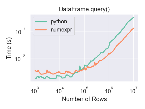
You will only see the performance benefits of using the numexpr engine with DataFrame.query() if your frame has more than approximately 100,000 rows.

This plot was created using a DataFrame with 3 columns each containing floating point values generated using numpy.random.randn().

In [296]: df = pd.DataFrame(np.random.randn(8, 4), .....: index=dates, columns=['A', 'B', 'C', 'D']) .....:

In [297]: df2 = df.copy()

Duplicate data#

If you want to identify and remove duplicate rows in a DataFrame, there are two methods that will help: duplicated and drop_duplicates. Each takes as an argument the columns to use to identify duplicated rows.

• duplicated returns a boolean vector whose length is the number of rows, and which indicates whether a row is duplicated.
• drop_duplicates removes duplicate rows.

By default, the first observed row of a duplicate set is considered unique, but each method has a keep parameter to specify targets to be kept.

• keep='first' (default): mark / drop duplicates except for the first occurrence.
• keep='last': mark / drop duplicates except for the last occurrence.
• keep=False: mark / drop all duplicates.

In [298]: df2 = pd.DataFrame({'a': ['one', 'one', 'two', 'two', 'two', 'three', 'four'], .....: 'b': ['x', 'y', 'x', 'y', 'x', 'x', 'x'], .....: 'c': np.random.randn(7)}) .....:

In [299]: df2 Out[299]: a b c 0 one x -1.067137 1 one y 0.309500 2 two x -0.211056 3 two y -1.842023 4 two x -0.390820 5 three x -1.964475 6 four x 1.298329

In [300]: df2.duplicated('a') Out[300]: 0 False 1 True 2 False 3 True 4 True 5 False 6 False dtype: bool

In [301]: df2.duplicated('a', keep='last') Out[301]: 0 True 1 False 2 True 3 True 4 False 5 False 6 False dtype: bool

In [302]: df2.duplicated('a', keep=False) Out[302]: 0 True 1 True 2 True 3 True 4 True 5 False 6 False dtype: bool

In [303]: df2.drop_duplicates('a') Out[303]: a b c 0 one x -1.067137 2 two x -0.211056 5 three x -1.964475 6 four x 1.298329

In [304]: df2.drop_duplicates('a', keep='last') Out[304]: a b c 1 one y 0.309500 4 two x -0.390820 5 three x -1.964475 6 four x 1.298329

In [305]: df2.drop_duplicates('a', keep=False) Out[305]: a b c 5 three x -1.964475 6 four x 1.298329

Also, you can pass a list of columns to identify duplications.

In [306]: df2.duplicated(['a', 'b']) Out[306]: 0 False 1 False 2 False 3 False 4 True 5 False 6 False dtype: bool

In [307]: df2.drop_duplicates(['a', 'b']) Out[307]: a b c 0 one x -1.067137 1 one y 0.309500 2 two x -0.211056 3 two y -1.842023 5 three x -1.964475 6 four x 1.298329

To drop duplicates by index value, use Index.duplicated then perform slicing. The same set of options are available for the keep parameter.

In [308]: df3 = pd.DataFrame({'a': np.arange(6), .....: 'b': np.random.randn(6)}, .....: index=['a', 'a', 'b', 'c', 'b', 'a']) .....:

In [309]: df3 Out[309]: a b a 0 1.440455 a 1 2.456086 b 2 1.038402 c 3 -0.894409 b 4 0.683536 a 5 3.082764

In [310]: df3.index.duplicated() Out[310]: array([False, True, False, False, True, True])

In [311]: df3[~df3.index.duplicated()] Out[311]: a b a 0 1.440455 b 2 1.038402 c 3 -0.894409

In [312]: df3[~df3.index.duplicated(keep='last')] Out[312]: a b c 3 -0.894409 b 4 0.683536 a 5 3.082764

In [313]: df3[~df3.index.duplicated(keep=False)] Out[313]: a b c 3 -0.894409

Dictionary-like get() method#

Each of Series or DataFrame have a get method which can return a default value.

In [314]: s = pd.Series([1, 2, 3], index=['a', 'b', 'c'])

In [315]: s.get('a') # equivalent to s['a'] Out[315]: np.int64(1)

In [316]: s.get('x', default=-1) Out[316]: -1

Looking up values by index/column labels#

Sometimes you want to extract a set of values given a sequence of row labels and column labels, this can be achieved by pandas.factorize and NumPy indexing. For instance:

In [317]: df = pd.DataFrame({'col': ["A", "A", "B", "B"], .....: 'A': [80, 23, np.nan, 22], .....: 'B': [80, 55, 76, 67]}) .....:

In [318]: df Out[318]: col A B 0 A 80.0 80 1 A 23.0 55 2 B NaN 76 3 B 22.0 67

In [319]: idx, cols = pd.factorize(df['col'])

In [320]: df.reindex(cols, axis=1).to_numpy()[np.arange(len(df)), idx] Out[320]: array([80., 23., 76., 67.])

Formerly this could be achieved with the dedicated DataFrame.lookup method which was deprecated in version 1.2.0 and removed in version 2.0.0.

Index objects#

The pandas Index class and its subclasses can be viewed as implementing an ordered multiset. Duplicates are allowed.

Index also provides the infrastructure necessary for lookups, data alignment, and reindexing. The easiest way to create anIndex directly is to pass a list or other sequence toIndex:

In [321]: index = pd.Index(['e', 'd', 'a', 'b'])

In [322]: index Out[322]: Index(['e', 'd', 'a', 'b'], dtype='object')

In [323]: 'd' in index Out[323]: True

or using numbers:

In [324]: index = pd.Index([1, 5, 12])

In [325]: index Out[325]: Index([1, 5, 12], dtype='int64')

In [326]: 5 in index Out[326]: True

If no dtype is given, Index tries to infer the dtype from the data. It is also possible to give an explicit dtype when instantiating an Index:

In [327]: index = pd.Index(['e', 'd', 'a', 'b'], dtype="string")

In [328]: index Out[328]: Index(['e', 'd', 'a', 'b'], dtype='string')

In [329]: index = pd.Index([1, 5, 12], dtype="int8")

In [330]: index Out[330]: Index([1, 5, 12], dtype='int8')

In [331]: index = pd.Index([1, 5, 12], dtype="float32")

In [332]: index Out[332]: Index([1.0, 5.0, 12.0], dtype='float32')

You can also pass a name to be stored in the index:

In [333]: index = pd.Index(['e', 'd', 'a', 'b'], name='something')

In [334]: index.name Out[334]: 'something'

The name, if set, will be shown in the console display:

In [335]: index = pd.Index(list(range(5)), name='rows')

In [336]: columns = pd.Index(['A', 'B', 'C'], name='cols')

In [337]: df = pd.DataFrame(np.random.randn(5, 3), index=index, columns=columns)

In [338]: df Out[338]: cols A B C rows
0 1.295989 -1.051694 1.340429 1 -2.366110 0.428241 0.387275 2 0.433306 0.929548 0.278094 3 2.154730 -0.315628 0.264223 4 1.126818 1.132290 -0.353310

In [339]: df['A'] Out[339]: rows 0 1.295989 1 -2.366110 2 0.433306 3 2.154730 4 1.126818 Name: A, dtype: float64

Setting metadata#

Indexes are “mostly immutable”, but it is possible to set and change theirname attribute. You can use the rename, set_names to set these attributes directly, and they default to returning a copy.

See Advanced Indexing for usage of MultiIndexes.

In [340]: ind = pd.Index([1, 2, 3])

In [341]: ind.rename("apple") Out[341]: Index([1, 2, 3], dtype='int64', name='apple')

In [342]: ind Out[342]: Index([1, 2, 3], dtype='int64')

In [343]: ind = ind.set_names(["apple"])

In [344]: ind.name = "bob"

In [345]: ind Out[345]: Index([1, 2, 3], dtype='int64', name='bob')

set_names, set_levels, and set_codes also take an optionallevel argument

In [346]: index = pd.MultiIndex.from_product([range(3), ['one', 'two']], names=['first', 'second'])

In [347]: index Out[347]: MultiIndex([(0, 'one'), (0, 'two'), (1, 'one'), (1, 'two'), (2, 'one'), (2, 'two')], names=['first', 'second'])

In [348]: index.levels[1] Out[348]: Index(['one', 'two'], dtype='object', name='second')

In [349]: index.set_levels(["a", "b"], level=1) Out[349]: MultiIndex([(0, 'a'), (0, 'b'), (1, 'a'), (1, 'b'), (2, 'a'), (2, 'b')], names=['first', 'second'])

Set operations on Index objects#

The two main operations are union and intersection. Difference is provided via the .difference() method.

In [350]: a = pd.Index(['c', 'b', 'a'])

In [351]: b = pd.Index(['c', 'e', 'd'])

In [352]: a.difference(b) Out[352]: Index(['a', 'b'], dtype='object')

Also available is the symmetric_difference operation, which returns elements that appear in either idx1 or idx2, but not in both. This is equivalent to the Index created by idx1.difference(idx2).union(idx2.difference(idx1)), with duplicates dropped.

In [353]: idx1 = pd.Index([1, 2, 3, 4])

In [354]: idx2 = pd.Index([2, 3, 4, 5])

In [355]: idx1.symmetric_difference(idx2) Out[355]: Index([1, 5], dtype='int64')

Note

The resulting index from a set operation will be sorted in ascending order.

When performing Index.union() between indexes with different dtypes, the indexes must be cast to a common dtype. Typically, though not always, this is object dtype. The exception is when performing a union between integer and float data. In this case, the integer values are converted to float

In [356]: idx1 = pd.Index([0, 1, 2])

In [357]: idx2 = pd.Index([0.5, 1.5])

In [358]: idx1.union(idx2) Out[358]: Index([0.0, 0.5, 1.0, 1.5, 2.0], dtype='float64')

Missing values#

Important

Even though Index can hold missing values (NaN), it should be avoided if you do not want any unexpected results. For example, some operations exclude missing values implicitly.

Index.fillna fills missing values with specified scalar value.

In [359]: idx1 = pd.Index([1, np.nan, 3, 4])

In [360]: idx1 Out[360]: Index([1.0, nan, 3.0, 4.0], dtype='float64')

In [361]: idx1.fillna(2) Out[361]: Index([1.0, 2.0, 3.0, 4.0], dtype='float64')

In [362]: idx2 = pd.DatetimeIndex([pd.Timestamp('2011-01-01'), .....: pd.NaT, .....: pd.Timestamp('2011-01-03')]) .....:

In [363]: idx2 Out[363]: DatetimeIndex(['2011-01-01', 'NaT', '2011-01-03'], dtype='datetime64[s]', freq=None)

In [364]: idx2.fillna(pd.Timestamp('2011-01-02')) Out[364]: DatetimeIndex(['2011-01-01', '2011-01-02', '2011-01-03'], dtype='datetime64[s]', freq=None)

Set / reset index#

Occasionally you will load or create a data set into a DataFrame and want to add an index after you’ve already done so. There are a couple of different ways.

Set an index#

DataFrame has a set_index() method which takes a column name (for a regular Index) or a list of column names (for a MultiIndex). To create a new, re-indexed DataFrame:

In [365]: data = pd.DataFrame({'a': ['bar', 'bar', 'foo', 'foo'], .....: 'b': ['one', 'two', 'one', 'two'], .....: 'c': ['z', 'y', 'x', 'w'], .....: 'd': [1., 2., 3, 4]}) .....:

In [366]: data Out[366]: a b c d 0 bar one z 1.0 1 bar two y 2.0 2 foo one x 3.0 3 foo two w 4.0

In [367]: indexed1 = data.set_index('c')

In [368]: indexed1 Out[368]: a b d c
z bar one 1.0 y bar two 2.0 x foo one 3.0 w foo two 4.0

In [369]: indexed2 = data.set_index(['a', 'b'])

In [370]: indexed2 Out[370]: c d a b
bar one z 1.0 two y 2.0 foo one x 3.0 two w 4.0

The append keyword option allow you to keep the existing index and append the given columns to a MultiIndex:

In [371]: frame = data.set_index('c', drop=False)

In [372]: frame = frame.set_index(['a', 'b'], append=True)

In [373]: frame Out[373]: c d c a b
z bar one z 1.0 y bar two y 2.0 x foo one x 3.0 w foo two w 4.0

Other options in set_index allow you not drop the index columns.

In [374]: data.set_index('c', drop=False) Out[374]: a b c d c
z bar one z 1.0 y bar two y 2.0 x foo one x 3.0 w foo two w 4.0

Reset the index#

As a convenience, there is a new function on DataFrame calledreset_index() which transfers the index values into the DataFrame’s columns and sets a simple integer index. This is the inverse operation of set_index().

In [375]: data Out[375]: a b c d 0 bar one z 1.0 1 bar two y 2.0 2 foo one x 3.0 3 foo two w 4.0

In [376]: data.reset_index() Out[376]: index a b c d 0 0 bar one z 1.0 1 1 bar two y 2.0 2 2 foo one x 3.0 3 3 foo two w 4.0

The output is more similar to a SQL table or a record array. The names for the columns derived from the index are the ones stored in the names attribute.

You can use the level keyword to remove only a portion of the index:

In [377]: frame Out[377]: c d c a b
z bar one z 1.0 y bar two y 2.0 x foo one x 3.0 w foo two w 4.0

In [378]: frame.reset_index(level=1) Out[378]: a c d c b
z one bar z 1.0 y two bar y 2.0 x one foo x 3.0 w two foo w 4.0

reset_index takes an optional parameter drop which if true simply discards the index, instead of putting index values in the DataFrame’s columns.

Why does assignment fail when using chained indexing?#

Copy-on-Write is the new default with pandas 3.0. This means that chained indexing will never work. See this sectionfor more context.