PACE — PyDAP tutorial (original) (raw)

PACE#

This notebook demonstrates access to PACE Ocean Color Data. Broad information about the dataset can be found on the PACE website (see here)

Requirements to run this notebook

1. Have an Earth Data Login account
2. Have a Bearer Token.

You can also use username/password method described in Authentication, instead of the token approach.

Objectives

Use pydap’s client API to demonstrate

• Access to NASA’s EarthData in the cloud via the use of tokens.
• Access/download PACE data with an OPeNDAP URL and pydap’s client.
• Construct a Constraint Expression.
• Speed up the workflow by exploiting OPeNDAP’s data-proximate subsetting to access and download only subset of the original data.

Author: Miguel Jimenez-Urias, ‘24

import matplotlib.pyplot as plt import numpy as np from pydap.net import create_session from pydap.client import open_url import cartopy.crs as ccrs import xarray as xr

Access EARTHDATA#

The PACE OPeNDAP data catalog can be found here. Data only starts in 2024.

slow download URL / higher resolution

url_DAP4 = "http://oceandata.sci.gsfc.nasa.gov/opendap/PACE_OCI/L3SMI/2024/0310/PACE_OCI.20240310.L3m.DAY.CHL.V2_0.chlor_a.4km.NRT.nc"

Use .netrc credentials#

These are recovered automatically

my_session = create_session()

Alternative Token Approach#

session_extra = {"token": "YourToken"}

initialize a requests.session object with the token headers. All handled by pydap.

my_session = create_session(session_kwargs=session_extra)

%%time ds_full = open_url(url_DAP4, session=my_session, protocol='dap4')

CPU times: user 42.1 ms, sys: 7.23 ms, total: 49.3 ms Wall time: 937 ms

.PACE_OCI.20240310.L3m.DAY.CHL.V2_0.chlor_a.4km.NRT.nc ├──lat ├──lon ├──chlor_a └──palette

Note

PyDAP accesses the remote dataset’s metadata, and no data has been downloaded yet!

ds_full['chlor_a'].attributes

{'long_name': 'Chlorophyll Concentration, OCI Algorithm', 'units': 'mg m^-3', 'standard_name': 'mass_concentration_of_chlorophyll_in_sea_water', '_FillValue': -32767.0, 'valid_min': 0.00100000005, 'valid_max': 100.0, 'reference': 'Hu, C., Lee Z., and Franz, B.A. (2012). Chlorophyll-a algorithms for oligotrophic oceans: A novel approach based on three-band reflectance difference, J. Geophys. Res., 117, C01011, doi:10.1029/2011JC007395.', 'display_scale': 'log', 'display_min': 0.00999999978, 'display_max': 20.0, 'Maps': ('/lat', '/lon')}

print('uncompressed dataset size [GBs]: ', ds_full.nbytes / 1e9)

uncompressed dataset size [GBs]: 0.149351808

print('uncompressed dataset size [GBs]: ', ds_full['chlor_a'].nbytes / 1e9)

uncompressed dataset size [GBs]: 0.1492992

Download data by indexing the array#

When downloading, it is important to verify and check any necessary decoding in order to make sense of the data, in particular when trying to define a subset region of interest by latitude and longitude ranges. And so, we download latitude and longitude. each a one-dimensional array, thus keeping at a minimum the download amount.

Decoding data values:

xarray decodes time and spatial values internally by default, everytime one accesses the data values, whereas currently there is no such method within pydap to do so. But it is often useful to understand how this works internally, and what type of parameters are used for decoding. Because OPeNDAP is based on the NetCDF data model, it if a CF-compliant software. Below are some of the most used metadata attributes associated for decoding data:

CF - Conventions

In OPeNDAP’s metadata rich datasets, each contains standard attributes used to describe missing data, units in which the data is presented, and any stretching/scaling of the values.

• standard name
• units
• _FillValue
• scale_factor
• off_set

Below is a simple function that decodes the spatial values within the array:

def decode(variable) -> np.ndarray: """Decodes the variable BaseType according with atributes: _FillValue scale_factor

Parameters:
    variable: BaseType (pydap model)
"""
scale_factor = 1
_Fillvalue = None

if 'scale_factor' in variable.attributes:
    scale_factor = variable.scale_factor
if '_FillValue' in variable.attributes:
    data = np.where(variable.data == variable._FillValue, np.nan, variable.data)    
else:
    data = variable.data
return scale_factor * data

Download one-dimensional lat and lon values#

To make sense of these, we make sure to decode their values

lon = decode(ds_full['lon'][:]) lat = decode(ds_full['lat'][:])

print("Size of the latitude array ", lat.shape)

Size of the latitude array (4320,)

print("Spatial range of values ", (lat.min(), lat.max()))

Spatial range of values (np.float32(-89.97917), np.float32(89.979164))

print("Size of the longitude array ", lat.shape)

Size of the longitude array (4320,)

print("Spatial range of values ", (lon.min(), lon.max()))

Spatial range of values (np.float32(-179.97917), np.float32(179.97917))

Warning

Not all array values of lat/lon coordinates are monotonic. Always make sure that is the case, even when data is Level 3 or Level 4

Define area / subset of interest#

It is good practice to perform some exploratory data analysis to reduce the size of the download. Below we identify the spatial index that define our coverage, and will use that to index the array, and only download that subset.

Min/max of lon values

minLon, maxLon = -96, 10

Min/Max of lat values

minLat, maxLat = 6, 70

iLon = np.where((lon>minLon)&(lon < maxLon))[0] iLat= np.where((lat>minLat)&(lat < maxLat))[0]

Visual Inspection of coordinate arrays#

plt.figure(figsize=(12,4)) plt.subplot(121) plt.plot(lon, 'k--', alpha=0.75) plt.plot(iLon,lon[iLon], 'r', lw=6) plt.xlabel('x-indexes of original remote file') plt.ylabel("Longitudes") plt.subplot(122) plt.plot(lat,'k--', alpha=0.75) plt.plot(iLat,lat[iLat], 'r', lw=6) plt.xlabel('y-indexes of original remote file') plt.ylabel("Latitude") plt.show()

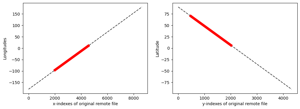
Fig 1. Lon and Lat values are continuous, and only cover data/region of interest.

Download only the subset#

and decode the values of the variable of interest.

%%time CHLOR_A = decode(ds_full['chlor_a'][iLat[0]:iLat[-1],iLon[0]:iLon[-1]])

CPU times: user 152 ms, sys: 72.8 ms, total: 225 ms Wall time: 1.67 s

print("Original size of array: ", ds_full['chlor_a'].shape)

Original size of array: (4320, 8640)

print("Size of downloaded subset: ",CHLOR_A.shape)

Size of downloaded subset: (1535, 2543)

Lon, Lat = np.meshgrid(lon[iLon[0]:iLon[-1]], lat[iLat[0]:iLat[-1]])

plt.figure(figsize=(25, 8)) ax = plt.axes(projection=ccrs.PlateCarree()) ax.set_global() ax.coastlines() plt.contourf(Lon, Lat, np.log(CHLOR_A), 400, cmap='nipy_spectral') plt.colorbar().set_label(ds_full['chlor_a'].name + ' ['+ds_full['chlor_a'].units+']');

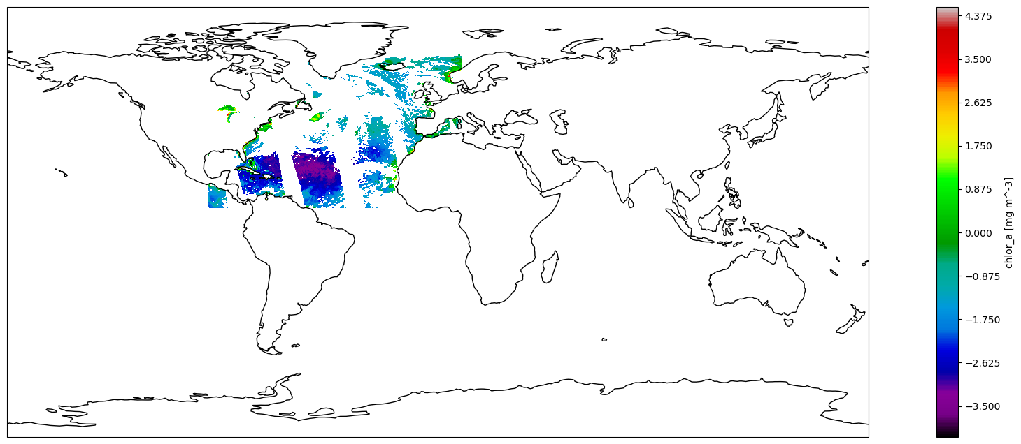
Fig 2. An approach to visually subset the global Chlorophyll A concentration. This approach allows to extract index values to construct the Constraint Expression and add it to the URL.

plt.figure(figsize=(25, 8)) ax = plt.axes(projection=ccrs.PlateCarree()) ax.coastlines() plt.contourf(Lon, Lat, np.log(CHLOR_A), 400, cmap='nipy_spectral') plt.colorbar().set_label(ds_full['chlor_a'].name + ' ['+ds_full['chlor_a'].units+']') plt.show()

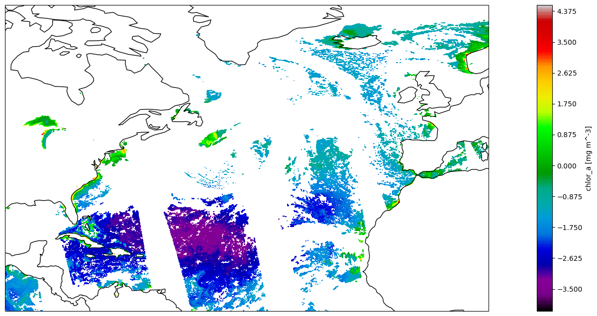
Fig 3. Same as in Figure 2, but now the plot shows only where data was downloaded.