Interactive visualization of PyTensor compute graphs — PyTensor dev documentation (original) (raw)

Guide#

Requirements#

d3viz requires the pydotpackage. Install it with pip:

Like PyTensor’s printing module, d3vizrequires graphviz binary to be available.

Overview#

d3viz extends PyTensor’s printing module to interactively visualize compute graphs. Instead of creating a static picture, it creates an HTML file, which can be opened with current web-browsers. d3viz allows

• to zoom to different regions and to move graphs via drag and drop,
• to position nodes both manually and automatically,
• to retrieve additional information about nodes and edges such as their data type or definition in the source code,
• to edit node labels,
• to visualizing profiling information, and
• to explore nested graphs such as OpFromGraph nodes.

As an example, consider the following multilayer perceptron with one hidden layer and a softmax output layer.

import pytensor import pytensor.tensor as pt import numpy as np

ninputs = 1000 nfeatures = 100 noutputs = 10 nhiddens = 50

rng = np.random.default_rng(0) x = pt.dmatrix('x') wh = pytensor.shared(rng.normal(0, 1, (nfeatures, nhiddens)), borrow=True) bh = pytensor.shared(np.zeros(nhiddens), borrow=True) h = pt.sigmoid(pt.dot(x, wh) + bh)

wy = pytensor.shared(rng.normal(0, 1, (nhiddens, noutputs))) by = pytensor.shared(np.zeros(noutputs), borrow=True) y = pt.special.softmax(pt.dot(h, wy) + by)

predict = pytensor.function([x], y)

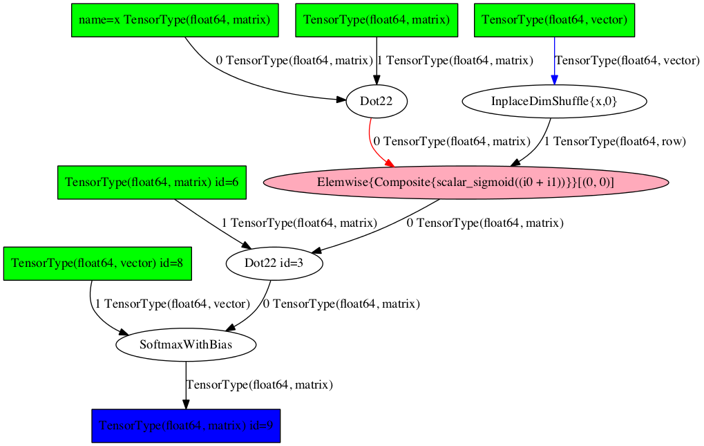
The function predict outputs the probability of 10 classes. You can visualize it with pytensor.printing.pydotprint() as follows:

from pytensor.printing import pydotprint from pathlib import Path

Path("examples").mkdir(exist_ok=True) pydotprint(predict, 'examples/mlp.png')

The output file is available at examples/mlp.png

from IPython.display import Image Image('./examples/mlp.png', width='80%')

To visualize it interactively, import pytensor.d3viz.d3viz.d3viz() from the the pytensor.d3viz.d3viz module, which can be called as before:

import pytensor.d3viz as d3v d3v.d3viz(predict, 'examples/mlp.html')

Open visualization!

When you open the output file mlp.html in your web-browser, you will see an interactive visualization of the compute graph. You can move the whole graph or single nodes via drag and drop, and zoom via the mouse wheel. When you move the mouse cursor over a node, a window will pop up that displays detailed information about the node, such as its data type or definition in the source code. When you left-click on a node and select Edit, you can change the predefined node label. If you are dealing with a complex graph with many nodes, the default node layout may not be perfect. In this case, you can press the Release nodebutton in the top-left corner to automatically arrange nodes. To reset nodes to their default position, press the Reset nodes button.

You can also display the interactive graph inline in IPython using IPython.display.IFrame:

from IPython.display import IFrame d3v.d3viz(predict, 'examples/mlp.html') IFrame('examples/mlp.html', width=700, height=500)

Currently if you use display.IFrame you still have to create a file, and this file can’t be outside notebooks root (e.g. usually it can’t be in /tmp/).

Profiling#

PyTensor allows function profiling via the profile=True flag. After at least one function call, the compute time of each node can be printed in text form with debugprint. However, analyzing complex graphs in this way can be cumbersome.

d3viz can visualize the same timing information graphically, and hence help to spot bottlenecks in the compute graph more easily! To begin with, we will redefine the predict function, this time by using profile=True flag. Afterwards, we capture the runtime on random data:

predict_profiled = pytensor.function([x], y, profile=True)

x_val = rng.normal(0, 1, (ninputs, nfeatures)) y_val = predict_profiled(x_val)

d3v.d3viz(predict_profiled, 'examples/mlp2.html')

Open visualization!

When you open the HTML file in your browser, you will find an additionalToggle profile colors button in the menu bar. By clicking on it, nodes will be colored by their compute time, where red corresponds to a high compute time. You can read out the exact timing information of a node by moving the cursor over it.

Different output formats#

Internally, d3viz represents a compute graph in the Graphviz DOT language, using thepydot package, and defines a front-end based on the d3.js library to visualize it. However, any other Graphviz front-end can be used, which allows to export graphs to different formats.

formatter = d3v.formatting.PyDotFormatter() pydot_graph = formatter(predict_profiled)

pydot_graph.write_png('examples/mlp2.png'); pydot_graph.write_png('examples/mlp2.pdf');

Image('./examples/mlp2.png')

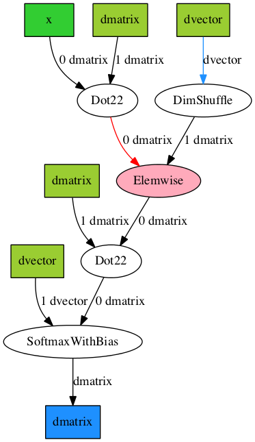
Here, we used the pytensor.d3viz.formatting.PyDotFormatter class to convert the compute graph into a pydot graph, and created aPNG and PDFfile. You can find all output formats supported by Graphviz here.

OpFromGraph nodes#

An OpFromGraph node defines a new operation, which can be called with different inputs at different places in the compute graph. Each OpFromGraphnode defines a nested graph, which will be visualized accordingly by d3viz.

x, y, z = pt.scalars('xyz') e = pt.sigmoid((x + y + z)**2) op = pytensor.compile.builders.OpFromGraph([x, y, z], [e])

e2 = op(x, y, z) + op(z, y, x) f = pytensor.function([x, y, z], e2)

d3v.d3viz(f, 'examples/ofg.html')

Open visualization!

In this example, an operation with three inputs is defined, which is used to build a function that calls this operations twice, each time with different input arguments.

In the d3viz visualization, you will find two OpFromGraph nodes, which correspond to the two OpFromGraph calls. When you double click on one of them, the nested graph appears with the correct mapping of its input arguments. You can move it around by drag and drop in the shaded area, and close it again by double-click.

An OpFromGraph operation can be composed of further OpFromGraph operations, which will be visualized as nested graphs as you can see in the following example.

x, y, z = pt.scalars('xyz') e = x * y op = pytensor.compile.builders.OpFromGraph([x, y], [e]) e2 = op(x, y) + z op2 = pytensor.compile.builders.OpFromGraph([x, y, z], [e2]) e3 = op2(x, y, z) + z f = pytensor.function([x, y, z], [e3])

d3v.d3viz(f, 'examples/ofg2.html')

Open visualization!

Feedback#

If you have any problems or great ideas on how to improve d3viz, please let me know!

• Christof Angermueller
• cangermueller@gmail.com
• https://cangermueller.com

References#

d3viz module#

Dynamic visualization of PyTensor graphs.

Author: Christof Angermueller <cangermueller@gmail.com>

pytensor.d3viz.d3viz.d3viz(fct, outfile, copy_deps=True, *args, **kwargs)[source]#

Create HTML file with dynamic visualizing of an PyTensor function graph.

In the HTML file, the whole graph or single nodes can be moved by drag and drop. Zooming is possible via the mouse wheel. Detailed information about nodes and edges are displayed via mouse-over events. Node labels can be edited by selecting Edit from the context menu.

Input nodes are colored in green, output nodes in blue. Apply nodes are ellipses, and colored depending on the type of operation they perform.

Edges are black by default. If a node returns a view of an input, the input edge will be blue. If it returns a destroyed input, the edge will be red.

Parameters:

• fct (pytensor.compile.function.types.Function) – A compiled PyTensor function, variable, apply or a list of variables.
• outfile (Path | str) – Path to output HTML file.
• copy_deps (bool , optional) – Copy javascript and CSS dependencies to output directory.

Notes

This function accepts extra parameters which will be forwarded topytensor.d3viz.formatting.PyDotFormatter.

pytensor.d3viz.d3viz.d3write(fct, path, *args, **kwargs)[source]#

Convert PyTensor graph to pydot graph and write to dot file.

Parameters:

• fct (pytensor.compile.function.types.Function) – A compiled PyTensor function, variable, apply or a list of variables.
• path (str) – Path to output file

Notes

This function accepts extra parameters which will be forwarded topytensor.d3viz.formatting.PyDotFormatter.

pytensor.d3viz.d3viz.replace_patterns(x, replace)[source]#

Replace replace in string x.

Parameters:

• s (str) – String on which function is applied
• replace (dict) – key, value pairs where key is a regular expression and value a string by which key is replaced

pytensor.d3viz.d3viz.safe_json(obj)[source]#

Encode obj to JSON so that it can be embedded safely inside HTML.

Parameters:

obj (object) – object to serialize

PyDotFormatter#

class pytensor.d3viz.formatting.PyDotFormatter(compact=True)[source]#

Create pydot graph object from PyTensor function.

Parameters:

compact (bool) – if True, will remove intermediate variables without name.

node_colors[source]#

Color table of node types.

Type:

dict

apply_colors[source]#

Color table of apply nodes.

Type:

dict

shapes[source]#

Shape table of node types.

Type:

dict

__call__(fct, graph=None)[source]#

Create pydot graph from function.

Parameters:

• fct (pytensor.compile.function.types.Function) – A compiled PyTensor function, variable, apply or a list of variables.
• graph (pydot.Dot) – pydot graph to which nodes are added. Creates new one if undefined.

Returns:

Pydot graph of fct

Return type:

pydot.Dot