arviz.plot_forest — ArviZ dev documentation (original) (raw)
arviz.plot_forest(data, kind='forestplot', model_names=None, var_names=None, filter_vars=None, transform=None, coords=None, combined=False, combine_dims=None, hdi_prob=None, rope=None, quartiles=True, ess=False, r_hat=False, colors='cycle', textsize=None, linewidth=None, markersize=None, legend=True, labeller=None, ridgeplot_alpha=None, ridgeplot_overlap=2, ridgeplot_kind='auto', ridgeplot_truncate=True, ridgeplot_quantiles=None, figsize=None, ax=None, backend=None, backend_config=None, backend_kwargs=None, show=None)[source]#
Forest plot to compare HDI intervals from a number of distributions.
Generate forest or ridge plots to compare distributions from a model or list of models. Additionally, the function can display effective sample sizes (ess) and Rhats to visualize convergence diagnostics alongside the distributions.
Parameters:
dataInferenceData
Any object that can be converted to an arviz.InferenceData object Refer to documentation of arviz.convert_to_dataset() for details.
kind{“foresplot”, “ridgeplot”}, default “forestplot”
Specify the kind of plot:
- The
kind="forestplot"generates credible intervals, where the central points are the estimated posterior median, the thick lines are the central quartiles, and the thin lines represent the \(100\times(hdi\_prob)\%\) highest density intervals. - The
kind="ridgeplot"option generates density plots (kernel density estimate or histograms) in the same graph. Ridge plots can be configured to have different overlap, truncation bounds and quantile markers.
model_nameslist of str, optional
List with names for the models in the list of data. Useful when plotting more that one dataset.
var_nameslist of str, optional
Variables to be plotted. Prefix the variables by ~ when you want to exclude them from the plot. See this section for usage examples.
combine_dimsset_like of str, optional
List of dimensions to reduce. Defaults to reducing only the “chain” and “draw” dimensions. See this section for usage examples.
filter_vars{None, “like”, “regex”}, default None
If None (default), interpret var_names as the real variables names. If “like”, interpret var_names as substrings of the real variables names. If “regex”, interpret var_names as regular expressions on the real variables names. Seethis section for usage examples.
transformcallable(), optional
Function to transform data (defaults to None i.e.the identity function).
coordsdict, optional
Coordinates of var_names to be plotted. Passed to xarray.Dataset.sel(). See this section for usage examples.
Flag for combining multiple chains into a single chain. If False, chains will be plotted separately. See this section for usage examples.
hdi_probfloat, default 0.94
Plots highest posterior density interval for chosen percentage of density. See this section for usage examples.
ropelist, tuple or dictionary of {strtuples or lists}, optional
A dictionary of tuples with the lower and upper values of the Region Of Practical Equivalence. See this section for usage examples.
Flag for plotting the interquartile range, in addition to the hdi_prob intervals.
Flag for plotting Split R-hat statistics. Requires 2 or more chains.
Flag for plotting the effective sample size.
list with valid matplotlib colors, one color per model. Alternative a string can be passed. If the string is cycle, it will automatically chose a color per model from the matplotlibs cycle. If a single color is passed, eg ‘k’, ‘C2’, ‘red’ this color will be used for all models. Defaults to ‘cycle’.
textsizefloat, optional
Text size scaling factor for labels, titles and lines. If None it will be autoscaled based on figsize.
linewidthint, optional
Line width throughout. If None it will be autoscaled based on figsize.
markersizeint, optional
Markersize throughout. If None it will be autoscaled based on figsize.
legendbool, optional
Show a legend with the color encoded model information. Defaults to True, if there are multiple models.
labellerLabeller, optional
Class providing the method make_label_vert to generate the labels in the plot titles. Read the Label guide for more details and usage examples.
ridgeplot_alpha: float, optional
Transparency for ridgeplot fill. If ridgeplot_alpha=0, border is colored by model, otherwise a black outline is used.
ridgeplot_overlapfloat, default 2
Overlap height for ridgeplots.
ridgeplot_kindstr, optional
By default (“auto”) continuous variables are plotted using KDEs and discrete ones using histograms. To override this use “hist” to plot histograms and “density” for KDEs.
ridgeplot_truncatebool, default True
Whether to truncate densities according to the value of hdi_prob.
ridgeplot_quantileslist, optional
Quantiles in ascending order used to segment the KDE. Use [.25, .5, .75] for quartiles.
figsize(float, float), optional
Figure size. If None, it will be defined automatically.
axaxes, optional
matplotlib.axes.Axes or bokeh.plotting.Figure.
backend{“matplotlib”, “bokeh”}, default “matplotlib”
Select plotting backend.
backend_configdict, optional
Currently specifies the bounds to use for bokeh axes. Defaults to value set in rcParams.
backend_kwargsdict, optional
These are kwargs specific to the backend being used, passed tomatplotlib.pyplot.subplots() or bokeh.plotting.figure. For additional documentation check the plotting method of the backend.
showbool, optional
Call backend show function.
Returns:
1D ndarray of matplotlib Axes or bokeh_figures
See also
Plot Posterior densities in the style of John K. Kruschke’s book.
Generate KDE plots for continuous variables and histograms for discrete ones.
Create a data frame with summary statistics.
Examples
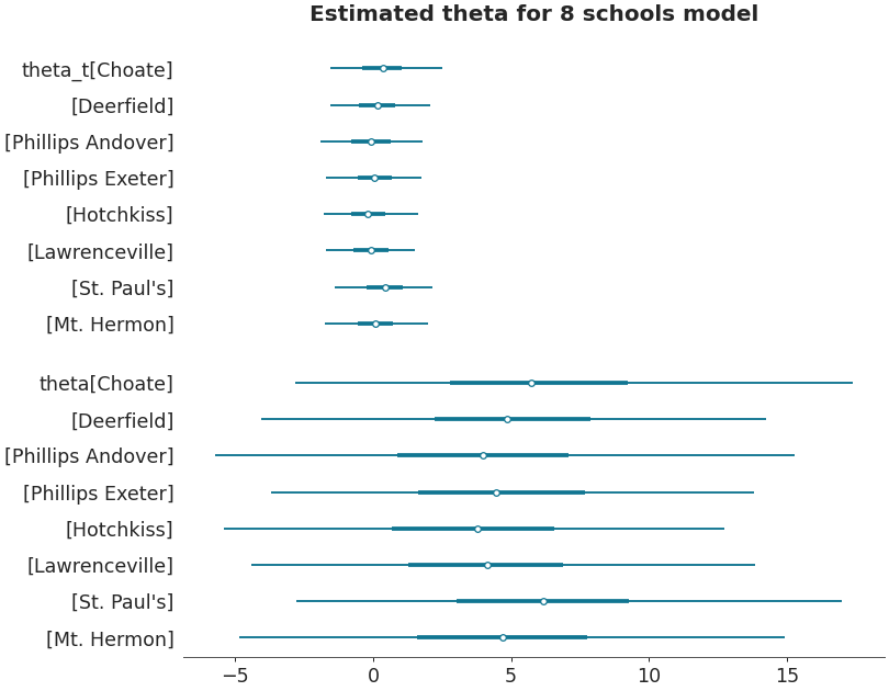
Forestplot
import arviz as az non_centered_data = az.load_arviz_data('non_centered_eight') axes = az.plot_forest(non_centered_data, kind='forestplot', var_names=["^the"], filter_vars="regex", combined=True, figsize=(9, 7)) axes[0].set_title('Estimated theta for 8 schools model')
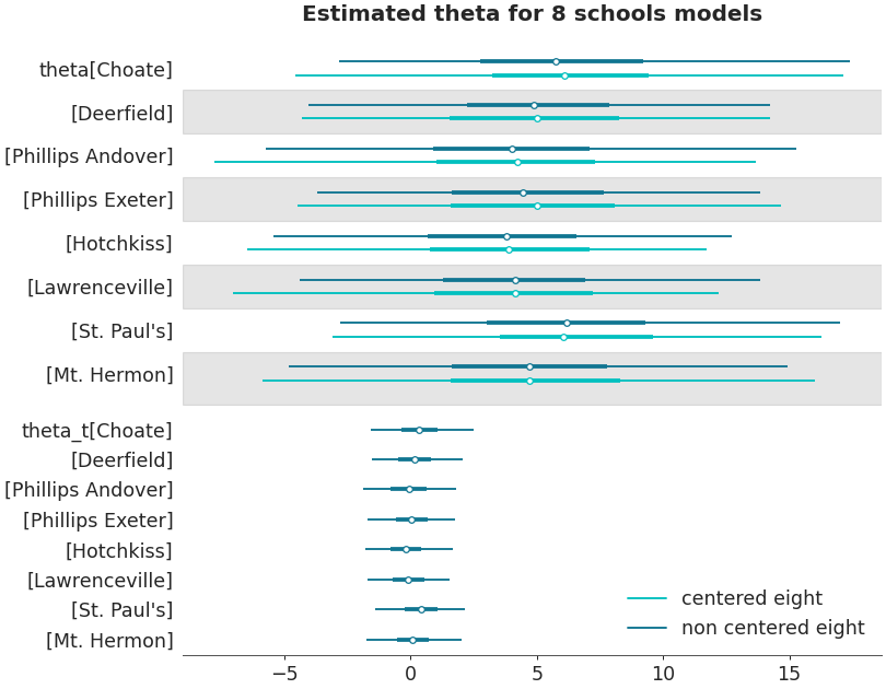
Forestplot with multiple datasets
centered_data = az.load_arviz_data('centered_eight') axes = az.plot_forest([non_centered_data, centered_data], model_names = ["non centered eight", "centered eight"], kind='forestplot', var_names=["^the"], filter_vars="regex", combined=True, figsize=(9, 7)) axes[0].set_title('Estimated theta for 8 schools models')
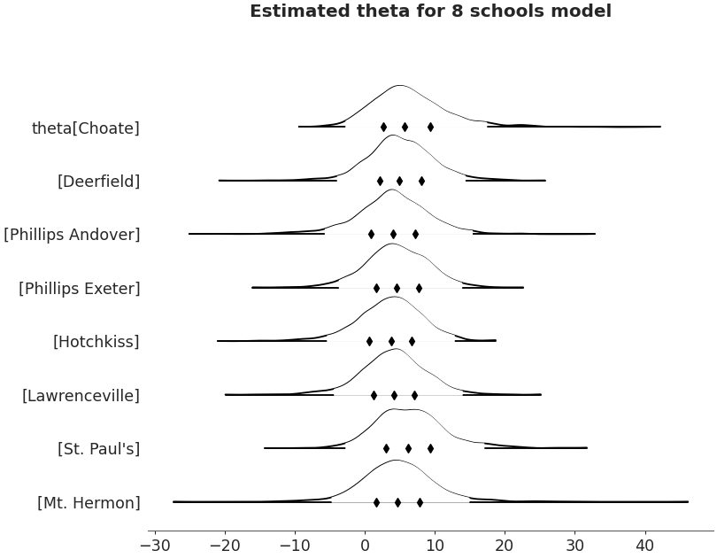
Ridgeplot
axes = az.plot_forest(non_centered_data, kind='ridgeplot', var_names=['theta'], combined=True, ridgeplot_overlap=3, colors='white', figsize=(9, 7)) axes[0].set_title('Estimated theta for 8 schools model')
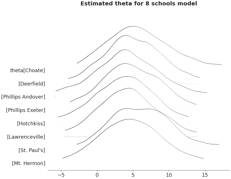
Ridgeplot non-truncated and with quantiles
axes = az.plot_forest(non_centered_data, kind='ridgeplot', var_names=['theta'], combined=True, ridgeplot_truncate=False, ridgeplot_quantiles=[.25, .5, .75], ridgeplot_overlap=0.7, colors='white', figsize=(9, 7)) axes[0].set_title('Estimated theta for 8 schools model')