Linear Regression Example — scikit-learn 0.20.4 documentation (original) (raw)
Note
Click here to download the full example code
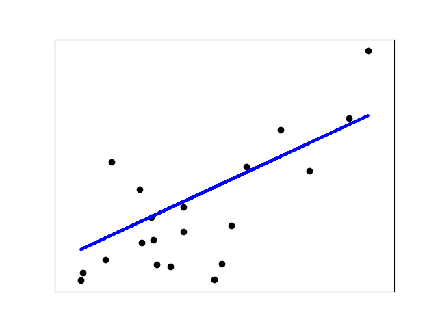
This example uses the only the first feature of the diabetes dataset, in order to illustrate a two-dimensional plot of this regression technique. The straight line can be seen in the plot, showing how linear regression attempts to draw a straight line that will best minimize the residual sum of squares between the observed responses in the dataset, and the responses predicted by the linear approximation.
The coefficients, the residual sum of squares and the variance score are also calculated.
Out:
Coefficients: [938.23786125] Mean squared error: 2548.07 Variance score: 0.47
print(doc)
Code source: Jaques Grobler
License: BSD 3 clause
import matplotlib.pyplot as plt import numpy as np from sklearn import datasets, linear_model from sklearn.metrics import mean_squared_error, r2_score
Load the diabetes dataset
diabetes = datasets.load_diabetes()
Use only one feature
diabetes_X = diabetes.data[:, np.newaxis, 2]
Split the data into training/testing sets
diabetes_X_train = diabetes_X[:-20] diabetes_X_test = diabetes_X[-20:]
Split the targets into training/testing sets
diabetes_y_train = diabetes.target[:-20] diabetes_y_test = diabetes.target[-20:]
Create linear regression object
regr = linear_model.LinearRegression()
Train the model using the training sets
regr.fit(diabetes_X_train, diabetes_y_train)
Make predictions using the testing set
diabetes_y_pred = regr.predict(diabetes_X_test)
The coefficients
print('Coefficients: \n', regr.coef_)
The mean squared error
print("Mean squared error: %.2f" % mean_squared_error(diabetes_y_test, diabetes_y_pred))
Explained variance score: 1 is perfect prediction
print('Variance score: %.2f' % r2_score(diabetes_y_test, diabetes_y_pred))
Plot outputs
plt.scatter(diabetes_X_test, diabetes_y_test, color='black') plt.plot(diabetes_X_test, diabetes_y_pred, color='blue', linewidth=3)
plt.xticks(()) plt.yticks(())
plt.show()
Total running time of the script: ( 0 minutes 0.164 seconds)