Theil-Sen Regression — scikit-learn 0.20.4 documentation (original) (raw)
Note
Click here to download the full example code
Computes a Theil-Sen Regression on a synthetic dataset.
See Theil-Sen estimator: generalized-median-based estimator for more information on the regressor.
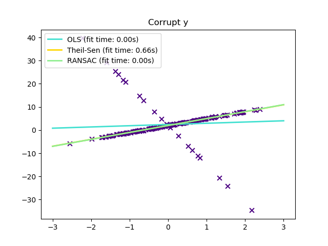
Compared to the OLS (ordinary least squares) estimator, the Theil-Sen estimator is robust against outliers. It has a breakdown point of about 29.3% in case of a simple linear regression which means that it can tolerate arbitrary corrupted data (outliers) of up to 29.3% in the two-dimensional case.
The estimation of the model is done by calculating the slopes and intercepts of a subpopulation of all possible combinations of p subsample points. If an intercept is fitted, p must be greater than or equal to n_features + 1. The final slope and intercept is then defined as the spatial median of these slopes and intercepts.
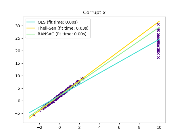
In certain cases Theil-Sen performs better than RANSAC which is also a robust method. This is illustrated in the second example below where outliers with respect to the x-axis perturb RANSAC. Tuning the residual_threshold parameter of RANSAC remedies this but in general a priori knowledge about the data and the nature of the outliers is needed. Due to the computational complexity of Theil-Sen it is recommended to use it only for small problems in terms of number of samples and features. For larger problems the max_subpopulation parameter restricts the magnitude of all possible combinations of p subsample points to a randomly chosen subset and therefore also limits the runtime. Therefore, Theil-Sen is applicable to larger problems with the drawback of losing some of its mathematical properties since it then works on a random subset.
Out:
Author: Florian Wilhelm -- florian.wilhelm@gmail.com
License: BSD 3 clause
import time import numpy as np import matplotlib.pyplot as plt from sklearn.linear_model import LinearRegression, TheilSenRegressor from sklearn.linear_model import RANSACRegressor
print(doc)
estimators = [('OLS', LinearRegression()), ('Theil-Sen', TheilSenRegressor(random_state=42)), ('RANSAC', RANSACRegressor(random_state=42)), ] colors = {'OLS': 'turquoise', 'Theil-Sen': 'gold', 'RANSAC': 'lightgreen'} lw = 2
Outliers only in the y direction
np.random.seed(0) n_samples = 200
Linear model y = 3*x + N(2, 0.1**2)
x = np.random.randn(n_samples) w = 3. c = 2. noise = 0.1 * np.random.randn(n_samples) y = w * x + c + noise
10% outliers
y[-20:] += -20 * x[-20:] X = x[:, np.newaxis]
plt.scatter(x, y, color='indigo', marker='x', s=40) line_x = np.array([-3, 3]) for name, estimator in estimators: t0 = time.time() estimator.fit(X, y) elapsed_time = time.time() - t0 y_pred = estimator.predict(line_x.reshape(2, 1)) plt.plot(line_x, y_pred, color=colors[name], linewidth=lw, label='%s (fit time: %.2fs)' % (name, elapsed_time))
plt.axis('tight') plt.legend(loc='upper left') plt.title("Corrupt y")
Outliers in the X direction
np.random.seed(0)
Linear model y = 3*x + N(2, 0.1**2)
x = np.random.randn(n_samples) noise = 0.1 * np.random.randn(n_samples) y = 3 * x + 2 + noise
10% outliers
x[-20:] = 9.9 y[-20:] += 22 X = x[:, np.newaxis]
plt.figure() plt.scatter(x, y, color='indigo', marker='x', s=40)
line_x = np.array([-3, 10]) for name, estimator in estimators: t0 = time.time() estimator.fit(X, y) elapsed_time = time.time() - t0 y_pred = estimator.predict(line_x.reshape(2, 1)) plt.plot(line_x, y_pred, color=colors[name], linewidth=lw, label='%s (fit time: %.2fs)' % (name, elapsed_time))
plt.axis('tight') plt.legend(loc='upper left') plt.title("Corrupt x") plt.show()
Total running time of the script: ( 0 minutes 1.579 seconds)