quantifying the quality of predictions — scikit-learn 0.20.4 documentation (original) (raw)
Finally, Dummy estimators are useful to get a baseline value of those metrics for random predictions.
3.3.1. The scoring parameter: defining model evaluation rules
Model selection and evaluation using tools, such asmodel_selection.GridSearchCV andmodel_selection.cross_val_score, take a scoring parameter that controls what metric they apply to the estimators evaluated.
3.3.1.1. Common cases: predefined values
For the most common use cases, you can designate a scorer object with thescoring parameter; the table below shows all possible values. All scorer objects follow the convention that higher return values are better than lower return values. Thus metrics which measure the distance between the model and the data, like metrics.mean_squared_error, are available as neg_mean_squared_error which return the negated value of the metric.
| Scoring | Function | Comment |
|---|---|---|
| Classification | ||
| ‘accuracy’ | metrics.accuracy_score | |
| ‘balanced_accuracy’ | metrics.balanced_accuracy_score | for binary targets |
| ‘average_precision’ | metrics.average_precision_score | |
| ‘brier_score_loss’ | metrics.brier_score_loss | |
| ‘f1’ | metrics.f1_score | for binary targets |
| ‘f1_micro’ | metrics.f1_score | micro-averaged |
| ‘f1_macro’ | metrics.f1_score | macro-averaged |
| ‘f1_weighted’ | metrics.f1_score | weighted average |
| ‘f1_samples’ | metrics.f1_score | by multilabel sample |
| ‘neg_log_loss’ | metrics.log_loss | requires predict_proba support |
| ‘precision’ etc. | metrics.precision_score | suffixes apply as with ‘f1’ |
| ‘recall’ etc. | metrics.recall_score | suffixes apply as with ‘f1’ |
| ‘roc_auc’ | metrics.roc_auc_score | |
| Clustering | ||
| ‘adjusted_mutual_info_score’ | metrics.adjusted_mutual_info_score | |
| ‘adjusted_rand_score’ | metrics.adjusted_rand_score | |
| ‘completeness_score’ | metrics.completeness_score | |
| ‘fowlkes_mallows_score’ | metrics.fowlkes_mallows_score | |
| ‘homogeneity_score’ | metrics.homogeneity_score | |
| ‘mutual_info_score’ | metrics.mutual_info_score | |
| ‘normalized_mutual_info_score’ | metrics.normalized_mutual_info_score | |
| ‘v_measure_score’ | metrics.v_measure_score | |
| Regression | ||
| ‘explained_variance’ | metrics.explained_variance_score | |
| ‘neg_mean_absolute_error’ | metrics.mean_absolute_error | |
| ‘neg_mean_squared_error’ | metrics.mean_squared_error | |
| ‘neg_mean_squared_log_error’ | metrics.mean_squared_log_error | |
| ‘neg_median_absolute_error’ | metrics.median_absolute_error | |
| ‘r2’ | metrics.r2_score |
Usage examples:
from sklearn import svm, datasets from sklearn.model_selection import cross_val_score iris = datasets.load_iris() X, y = iris.data, iris.target clf = svm.SVC(gamma='scale', random_state=0) cross_val_score(clf, X, y, scoring='recall_macro', ... cv=5)
array([0.96..., 0.96..., 0.96..., 0.93..., 1. ]) model = svm.SVC() cross_val_score(model, X, y, cv=5, scoring='wrong_choice') Traceback (most recent call last): ValueError: 'wrong_choice' is not a valid scoring value. Use sorted(sklearn.metrics.SCORERS.keys()) to get valid options.
Note
The values listed by the ValueError exception correspond to the functions measuring prediction accuracy described in the following sections. The scorer objects for those functions are stored in the dictionarysklearn.metrics.SCORERS.
3.3.1.2. Defining your scoring strategy from metric functions
The module sklearn.metrics also exposes a set of simple functions measuring a prediction error given ground truth and prediction:
- functions ending with
_scorereturn a value to maximize, the higher the better. - functions ending with
_erroror_lossreturn a value to minimize, the lower the better. When converting into a scorer object using make_scorer, set thegreater_is_betterparameter to False (True by default; see the parameter description below).
Metrics available for various machine learning tasks are detailed in sections below.
Many metrics are not given names to be used as scoring values, sometimes because they require additional parameters, such asfbeta_score. In such cases, you need to generate an appropriate scoring object. The simplest way to generate a callable object for scoring is by using make_scorer. That function converts metrics into callables that can be used for model evaluation.
One typical use case is to wrap an existing metric function from the library with non-default values for its parameters, such as the beta parameter for the fbeta_score function:
from sklearn.metrics import fbeta_score, make_scorer ftwo_scorer = make_scorer(fbeta_score, beta=2) from sklearn.model_selection import GridSearchCV from sklearn.svm import LinearSVC grid = GridSearchCV(LinearSVC(), param_grid={'C': [1, 10]}, ... scoring=ftwo_scorer, cv=5)
The second use case is to build a completely custom scorer object from a simple python function using make_scorer, which can take several parameters:
- the python function you want to use (
my_custom_loss_funcin the example below) - whether the python function returns a score (
greater_is_better=True, the default) or a loss (greater_is_better=False). If a loss, the output of the python function is negated by the scorer object, conforming to the cross validation convention that scorers return higher values for better models. - for classification metrics only: whether the python function you provided requires continuous decision certainties (
needs_threshold=True). The default value is False. - any additional parameters, such as
betaorlabelsin f1_score.
Here is an example of building custom scorers, and of using thegreater_is_better parameter:
import numpy as np def my_custom_loss_func(y_true, y_pred): ... diff = np.abs(y_true - y_pred).max() ... return np.log1p(diff) ...
score will negate the return value of my_custom_loss_func,
which will be np.log(2), 0.693, given the values for X
and y defined below.
score = make_scorer(my_custom_loss_func, greater_is_better=False) X = [[1], [1]] y = [0, 1] from sklearn.dummy import DummyClassifier clf = DummyClassifier(strategy='most_frequent', random_state=0) clf = clf.fit(X, y) my_custom_loss_func(clf.predict(X), y) 0.69... score(clf, X, y) -0.69...
3.3.1.3. Implementing your own scoring object
You can generate even more flexible model scorers by constructing your own scoring object from scratch, without using the make_scorer factory. For a callable to be a scorer, it needs to meet the protocol specified by the following two rules:
- It can be called with parameters
(estimator, X, y), whereestimatoris the model that should be evaluated,Xis validation data, andyis the ground truth target forX(in the supervised case) orNone(in the unsupervised case). - It returns a floating point number that quantifies the
estimatorprediction quality onX, with reference toy. Again, by convention higher numbers are better, so if your scorer returns loss, that value should be negated.
Note
Using custom scorers in functions where n_jobs > 1
While defining the custom scoring function alongside the calling function should work out of the box with the default joblib backend (loky), importing it from another module will be a more robust approach and work independently of the joblib backend.
For example, to use, n_jobs greater than 1 in the example below,custom_scoring_function function is saved in a user-created module (custom_scorer_module.py) and imported:
from custom_scorer_module import custom_scoring_function cross_val_score(model, ... X_train, ... y_train, ... scoring=make_scorer(custom_scoring_function, greater_is_better=False), ... cv=5, ... n_jobs=-1)
3.3.1.4. Using multiple metric evaluation
Scikit-learn also permits evaluation of multiple metrics in GridSearchCV,RandomizedSearchCV and cross_validate.
There are two ways to specify multiple scoring metrics for the scoringparameter:
- As an iterable of string metrics::
scoring = ['accuracy', 'precision']
- As a
dictmapping the scorer name to the scoring function::from sklearn.metrics import accuracy_score
from sklearn.metrics import make_scorer
scoring = {'accuracy': make_scorer(accuracy_score),
... 'prec': 'precision'}
Note that the dict values can either be scorer functions or one of the predefined metric strings.
Currently only those scorer functions that return a single score can be passed inside the dict. Scorer functions that return multiple values are not permitted and will require a wrapper to return a single metric:
from sklearn.model_selection import cross_validate from sklearn.metrics import confusion_matrix
A sample toy binary classification dataset
X, y = datasets.make_classification(n_classes=2, random_state=0) svm = LinearSVC(random_state=0) def tn(y_true, y_pred): return confusion_matrix(y_true, y_pred)[0, 0] def fp(y_true, y_pred): return confusion_matrix(y_true, y_pred)[0, 1] def fn(y_true, y_pred): return confusion_matrix(y_true, y_pred)[1, 0] def tp(y_true, y_pred): return confusion_matrix(y_true, y_pred)[1, 1] scoring = {'tp': make_scorer(tp), 'tn': make_scorer(tn), ... 'fp': make_scorer(fp), 'fn': make_scorer(fn)} cv_results = cross_validate(svm.fit(X, y), X, y, ... scoring=scoring, cv=5)
Getting the test set true positive scores
print(cv_results['test_tp'])
[10 9 8 7 8]Getting the test set false negative scores
print(cv_results['test_fn'])
[0 1 2 3 2]
3.3.2. Classification metrics
The sklearn.metrics module implements several loss, score, and utility functions to measure classification performance. Some metrics might require probability estimates of the positive class, confidence values, or binary decisions values. Most implementations allow each sample to provide a weighted contribution to the overall score, through the sample_weight parameter.
Some of these are restricted to the binary classification case:
| precision_recall_curve(y_true, probas_pred) | Compute precision-recall pairs for different probability thresholds |
|---|---|
| roc_curve(y_true, y_score[, pos_label, …]) | Compute Receiver operating characteristic (ROC) |
| balanced_accuracy_score(y_true, y_pred[, …]) | Compute the balanced accuracy |
Others also work in the multiclass case:
| cohen_kappa_score(y1, y2[, labels, weights, …]) | Cohen’s kappa: a statistic that measures inter-annotator agreement. |
|---|---|
| confusion_matrix(y_true, y_pred[, labels, …]) | Compute confusion matrix to evaluate the accuracy of a classification |
| hinge_loss(y_true, pred_decision[, labels, …]) | Average hinge loss (non-regularized) |
| matthews_corrcoef(y_true, y_pred[, …]) | Compute the Matthews correlation coefficient (MCC) |
Some also work in the multilabel case:
| accuracy_score(y_true, y_pred[, normalize, …]) | Accuracy classification score. |
|---|---|
| classification_report(y_true, y_pred[, …]) | Build a text report showing the main classification metrics |
| f1_score(y_true, y_pred[, labels, …]) | Compute the F1 score, also known as balanced F-score or F-measure |
| fbeta_score(y_true, y_pred, beta[, labels, …]) | Compute the F-beta score |
| hamming_loss(y_true, y_pred[, labels, …]) | Compute the average Hamming loss. |
| jaccard_similarity_score(y_true, y_pred[, …]) | Jaccard similarity coefficient score |
| log_loss(y_true, y_pred[, eps, normalize, …]) | Log loss, aka logistic loss or cross-entropy loss. |
| precision_recall_fscore_support(y_true, y_pred) | Compute precision, recall, F-measure and support for each class |
| precision_score(y_true, y_pred[, labels, …]) | Compute the precision |
| recall_score(y_true, y_pred[, labels, …]) | Compute the recall |
| zero_one_loss(y_true, y_pred[, normalize, …]) | Zero-one classification loss. |
And some work with binary and multilabel (but not multiclass) problems:
| average_precision_score(y_true, y_score[, …]) | Compute average precision (AP) from prediction scores |
|---|---|
| roc_auc_score(y_true, y_score[, average, …]) | Compute Area Under the Receiver Operating Characteristic Curve (ROC AUC) from prediction scores. |
In the following sub-sections, we will describe each of those functions, preceded by some notes on common API and metric definition.
3.3.2.1. From binary to multiclass and multilabel
Some metrics are essentially defined for binary classification tasks (e.g.f1_score, roc_auc_score). In these cases, by default only the positive label is evaluated, assuming by default that the positive class is labelled 1 (though this may be configurable through thepos_label parameter).
In extending a binary metric to multiclass or multilabel problems, the data is treated as a collection of binary problems, one for each class. There are then a number of ways to average binary metric calculations across the set of classes, each of which may be useful in some scenario. Where available, you should select among these using the average parameter.
"macro"simply calculates the mean of the binary metrics, giving equal weight to each class. In problems where infrequent classes are nonetheless important, macro-averaging may be a means of highlighting their performance. On the other hand, the assumption that all classes are equally important is often untrue, such that macro-averaging will over-emphasize the typically low performance on an infrequent class."weighted"accounts for class imbalance by computing the average of binary metrics in which each class’s score is weighted by its presence in the true data sample."micro"gives each sample-class pair an equal contribution to the overall metric (except as a result of sample-weight). Rather than summing the metric per class, this sums the dividends and divisors that make up the per-class metrics to calculate an overall quotient. Micro-averaging may be preferred in multilabel settings, including multiclass classification where a majority class is to be ignored."samples"applies only to multilabel problems. It does not calculate a per-class measure, instead calculating the metric over the true and predicted classes for each sample in the evaluation data, and returning their (sample_weight-weighted) average.- Selecting
average=Nonewill return an array with the score for each class.
While multiclass data is provided to the metric, like binary targets, as an array of class labels, multilabel data is specified as an indicator matrix, in which cell [i, j] has value 1 if sample i has label j and value 0 otherwise.
3.3.2.2. Accuracy score
The accuracy_score function computes theaccuracy, either the fraction (default) or the count (normalize=False) of correct predictions.
In multilabel classification, the function returns the subset accuracy. If the entire set of predicted labels for a sample strictly match with the true set of labels, then the subset accuracy is 1.0; otherwise it is 0.0.
If \(\hat{y}_i\) is the predicted value of the \(i\)-th sample and \(y_i\) is the corresponding true value, then the fraction of correct predictions over \(n_\text{samples}\) is defined as
\[\texttt{accuracy}(y, \hat{y}) = \frac{1}{n_\text{samples}} \sum_{i=0}^{n_\text{samples}-1} 1(\hat{y}_i = y_i)\]
where \(1(x)\) is the indicator function.
import numpy as np from sklearn.metrics import accuracy_score y_pred = [0, 2, 1, 3] y_true = [0, 1, 2, 3] accuracy_score(y_true, y_pred) 0.5 accuracy_score(y_true, y_pred, normalize=False) 2
In the multilabel case with binary label indicators:
accuracy_score(np.array([[0, 1], [1, 1]]), np.ones((2, 2))) 0.5
Example:
- See Test with permutations the significance of a classification scorefor an example of accuracy score usage using permutations of the dataset.
3.3.2.3. Balanced accuracy score
The balanced_accuracy_score function computes the balanced accuracy, which avoids inflated performance estimates on imbalanced datasets. It is the macro-average of recall scores per class or, equivalently, raw accuracy where each sample is weighted according to the inverse prevalence of its true class. Thus for balanced datasets, the score is equal to accuracy.
In the binary case, balanced accuracy is equal to the arithmetic mean ofsensitivity(true positive rate) and specificity (true negative rate), or the area under the ROC curve with binary predictions rather than scores.
If the classifier performs equally well on either class, this term reduces to the conventional accuracy (i.e., the number of correct predictions divided by the total number of predictions).
In contrast, if the conventional accuracy is above chance only because the classifier takes advantage of an imbalanced test set, then the balanced accuracy, as appropriate, will drop to \(\frac{1}{n\_classes}\).
The score ranges from 0 to 1, or when adjusted=True is used, it rescaled to the range \(\frac{1}{1 - n\_classes}\) to 1, inclusive, with performance at random scoring 0.
If \(y_i\) is the true value of the \(i\)-th sample, and \(w_i\)is the corresponding sample weight, then we adjust the sample weight to:
\[\hat{w}_i = \frac{w_i}{\sum_j{1(y_j = y_i) w_j}}\]
where \(1(x)\) is the indicator function. Given predicted \(\hat{y}_i\) for sample \(i\), balanced accuracy is defined as:
\[\texttt{balanced-accuracy}(y, \hat{y}, w) = \frac{1}{\sum{\hat{w}_i}} \sum_i 1(\hat{y}_i = y_i) \hat{w}_i\]
With adjusted=True, balanced accuracy reports the relative increase from\(\texttt{balanced-accuracy}(y, \mathbf{0}, w) = \frac{1}{n\_classes}\). In the binary case, this is also known as*Youden’s J statistic*, or informedness.
Note
The multiclass definition here seems the most reasonable extension of the metric used in binary classification, though there is no certain consensus in the literature:
- Our definition: [Mosley2013], [Kelleher2015] and [Guyon2015], where[Guyon2015] adopt the adjusted version to ensure that random predictions have a score of \(0\) and perfect predictions have a score of \(1\)..
- Class balanced accuracy as described in [Mosley2013]: the minimum between the precision and the recall for each class is computed. Those values are then averaged over the total number of classes to get the balanced accuracy.
- Balanced Accuracy as described in [Urbanowicz2015]: the average of sensitivity and specificity is computed for each class and then averaged over total number of classes.
References:
| [Guyon2015] | (1, 2) I. Guyon, K. Bennett, G. Cawley, H.J. Escalante, S. Escalera, T.K. Ho, N. Macià, B. Ray, M. Saeed, A.R. Statnikov, E. Viegas, Design of the 2015 ChaLearn AutoML Challenge, IJCNN 2015. |
|---|
| [Mosley2013] | (1, 2) L. Mosley, A balanced approach to the multi-class imbalance problem, IJCV 2010. |
|---|
| [Kelleher2015] | John. D. Kelleher, Brian Mac Namee, Aoife D’Arcy, Fundamentals of Machine Learning for Predictive Data Analytics: Algorithms, Worked Examples, and Case Studies, 2015. |
|---|
| [Urbanowicz2015] | Urbanowicz R.J., Moore, J.H. ExSTraCS 2.0: description and evaluation of a scalable learning classifier system, Evol. Intel. (2015) 8: 89. |
|---|
3.3.2.4. Cohen’s kappa
The function cohen_kappa_score computes Cohen’s kappa statistic. This measure is intended to compare labelings by different human annotators, not a classifier versus a ground truth.
The kappa score (see docstring) is a number between -1 and 1. Scores above .8 are generally considered good agreement; zero or lower means no agreement (practically random labels).
Kappa scores can be computed for binary or multiclass problems, but not for multilabel problems (except by manually computing a per-label score) and not for more than two annotators.
from sklearn.metrics import cohen_kappa_score y_true = [2, 0, 2, 2, 0, 1] y_pred = [0, 0, 2, 2, 0, 2] cohen_kappa_score(y_true, y_pred) 0.4285714285714286
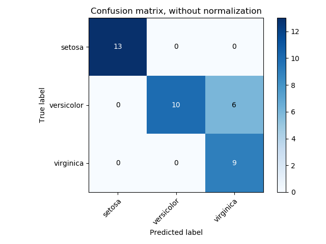
3.3.2.5. Confusion matrix
The confusion_matrix function evaluates classification accuracy by computing the confusion matrix with each row corresponding to the true class <https://en.wikipedia.org/wiki/Confusion_matrix>`_. (Wikipedia and other references may use different convention for axes.)
By definition, entry \(i, j\) in a confusion matrix is the number of observations actually in group \(i\), but predicted to be in group \(j\). Here is an example:
from sklearn.metrics import confusion_matrix y_true = [2, 0, 2, 2, 0, 1] y_pred = [0, 0, 2, 2, 0, 2] confusion_matrix(y_true, y_pred) array([[2, 0, 0], [0, 0, 1], [1, 0, 2]])
Here is a visual representation of such a confusion matrix (this figure comes from the Confusion matrix example):
For binary problems, we can get counts of true negatives, false positives, false negatives and true positives as follows:
y_true = [0, 0, 0, 1, 1, 1, 1, 1] y_pred = [0, 1, 0, 1, 0, 1, 0, 1] tn, fp, fn, tp = confusion_matrix(y_true, y_pred).ravel() tn, fp, fn, tp (2, 1, 2, 3)
Example:
- See Confusion matrixfor an example of using a confusion matrix to evaluate classifier output quality.
- See Recognizing hand-written digitsfor an example of using a confusion matrix to classify hand-written digits.
- See Classification of text documents using sparse featuresfor an example of using a confusion matrix to classify text documents.
3.3.2.6. Classification report
The classification_report function builds a text report showing the main classification metrics. Here is a small example with custom target_namesand inferred labels:
from sklearn.metrics import classification_report y_true = [0, 1, 2, 2, 0] y_pred = [0, 0, 2, 1, 0] target_names = ['class 0', 'class 1', 'class 2'] print(classification_report(y_true, y_pred, target_names=target_names)) precision recall f1-score support
 class 0       0.67      1.00      0.80         2
 class 1       0.00      0.00      0.00         1
 class 2       1.00      0.50      0.67         2
micro avg 0.60 0.60 0.60 5 macro avg 0.56 0.50 0.49 5 weighted avg 0.67 0.60 0.59 5
Example:
- See Recognizing hand-written digitsfor an example of classification report usage for hand-written digits.
- See Classification of text documents using sparse featuresfor an example of classification report usage for text documents.
- See Parameter estimation using grid search with cross-validationfor an example of classification report usage for grid search with nested cross-validation.
3.3.2.7. Hamming loss
The hamming_loss computes the average Hamming loss or Hamming distance between two sets of samples.
If \(\hat{y}_j\) is the predicted value for the \(j\)-th label of a given sample, \(y_j\) is the corresponding true value, and\(n_\text{labels}\) is the number of classes or labels, then the Hamming loss \(L_{Hamming}\) between two samples is defined as:
\[L_{Hamming}(y, \hat{y}) = \frac{1}{n_\text{labels}} \sum_{j=0}^{n_\text{labels} - 1} 1(\hat{y}_j \not= y_j)\]
where \(1(x)\) is the indicator function.
from sklearn.metrics import hamming_loss y_pred = [1, 2, 3, 4] y_true = [2, 2, 3, 4] hamming_loss(y_true, y_pred) 0.25
In the multilabel case with binary label indicators:
hamming_loss(np.array([[0, 1], [1, 1]]), np.zeros((2, 2))) 0.75
Note
In multiclass classification, the Hamming loss corresponds to the Hamming distance between y_true and y_pred which is similar to theZero one loss function. However, while zero-one loss penalizes prediction sets that do not strictly match true sets, the Hamming loss penalizes individual labels. Thus the Hamming loss, upper bounded by the zero-one loss, is always between zero and one, inclusive; and predicting a proper subset or superset of the true labels will give a Hamming loss between zero and one, exclusive.
3.3.2.8. Jaccard similarity coefficient score
The jaccard_similarity_score function computes the average (default) or sum of Jaccard similarity coefficients, also called the Jaccard index, between pairs of label sets.
The Jaccard similarity coefficient of the \(i\)-th samples, with a ground truth label set \(y_i\) and predicted label set\(\hat{y}_i\), is defined as
\[J(y_i, \hat{y}_i) = \frac{|y_i \cap \hat{y}_i|}{|y_i \cup \hat{y}_i|}.\]
In binary and multiclass classification, the Jaccard similarity coefficient score is equal to the classification accuracy.
import numpy as np from sklearn.metrics import jaccard_similarity_score y_pred = [0, 2, 1, 3] y_true = [0, 1, 2, 3] jaccard_similarity_score(y_true, y_pred) 0.5 jaccard_similarity_score(y_true, y_pred, normalize=False) 2
In the multilabel case with binary label indicators:
jaccard_similarity_score(np.array([[0, 1], [1, 1]]), np.ones((2, 2))) 0.75
3.3.2.9. Precision, recall and F-measures
Intuitively, precision is the ability of the classifier not to label as positive a sample that is negative, andrecall is the ability of the classifier to find all the positive samples.
The F-measure(\(F_\beta\) and \(F_1\) measures) can be interpreted as a weighted harmonic mean of the precision and recall. A\(F_\beta\) measure reaches its best value at 1 and its worst score at 0. With \(\beta = 1\), \(F_\beta\) and\(F_1\) are equivalent, and the recall and the precision are equally important.
The precision_recall_curve computes a precision-recall curve from the ground truth label and a score given by the classifier by varying a decision threshold.
The average_precision_score function computes theaverage precision(AP) from prediction scores. The value is between 0 and 1 and higher is better. AP is defined as
\[\text{AP} = \sum_n (R_n - R_{n-1}) P_n\]
where \(P_n\) and \(R_n\) are the precision and recall at the nth threshold. With random predictions, the AP is the fraction of positive samples.
References [Manning2008] and [Everingham2010] present alternative variants of AP that interpolate the precision-recall curve. Currently,average_precision_score does not implement any interpolated variant. References [Davis2006] and [Flach2015] describe why a linear interpolation of points on the precision-recall curve provides an overly-optimistic measure of classifier performance. This linear interpolation is used when computing area under the curve with the trapezoidal rule in auc.
Several functions allow you to analyze the precision, recall and F-measures score:
| average_precision_score(y_true, y_score[, …]) | Compute average precision (AP) from prediction scores |
|---|---|
| f1_score(y_true, y_pred[, labels, …]) | Compute the F1 score, also known as balanced F-score or F-measure |
| fbeta_score(y_true, y_pred, beta[, labels, …]) | Compute the F-beta score |
| precision_recall_curve(y_true, probas_pred) | Compute precision-recall pairs for different probability thresholds |
| precision_recall_fscore_support(y_true, y_pred) | Compute precision, recall, F-measure and support for each class |
| precision_score(y_true, y_pred[, labels, …]) | Compute the precision |
| recall_score(y_true, y_pred[, labels, …]) | Compute the recall |
Note that the precision_recall_curve function is restricted to the binary case. The average_precision_score function works only in binary classification and multilabel indicator format.
Examples:
- See Classification of text documents using sparse featuresfor an example of f1_score usage to classify text documents.
- See Parameter estimation using grid search with cross-validationfor an example of precision_score and recall_score usage to estimate parameters using grid search with nested cross-validation.
- See Precision-Recallfor an example of precision_recall_curve usage to evaluate classifier output quality.
References:
| [Manning2008] | C.D. Manning, P. Raghavan, H. Schütze, Introduction to Information Retrieval, 2008. |
|---|
| [Everingham2010] | M. Everingham, L. Van Gool, C.K.I. Williams, J. Winn, A. Zisserman,The Pascal Visual Object Classes (VOC) Challenge, IJCV 2010. |
|---|
| [Davis2006] | J. Davis, M. Goadrich, The Relationship Between Precision-Recall and ROC Curves, ICML 2006. |
|---|
| [Flach2015] | P.A. Flach, M. Kull, Precision-Recall-Gain Curves: PR Analysis Done Right, NIPS 2015. |
|---|
3.3.2.9.1. Binary classification
In a binary classification task, the terms ‘’positive’’ and ‘’negative’’ refer to the classifier’s prediction, and the terms ‘’true’’ and ‘’false’’ refer to whether that prediction corresponds to the external judgment (sometimes known as the ‘’observation’‘). Given these definitions, we can formulate the following table:
| | Actual class (observation) | | | | ---------------------------------- | -------------------------------------------- | ------------------------------------- | | Predicted class (expectation) | tp (true positive) Correct result | fp (false positive) Unexpected result | | fn (false negative) Missing result | tn (true negative) Correct absence of result | |
In this context, we can define the notions of precision, recall and F-measure:
\[\text{precision} = \frac{tp}{tp + fp},\]
\[\text{recall} = \frac{tp}{tp + fn},\]
\[F_\beta = (1 + \beta^2) \frac{\text{precision} \times \text{recall}}{\beta^2 \text{precision} + \text{recall}}.\]
Here are some small examples in binary classification:
from sklearn import metrics y_pred = [0, 1, 0, 0] y_true = [0, 1, 0, 1] metrics.precision_score(y_true, y_pred) 1.0 metrics.recall_score(y_true, y_pred) 0.5 metrics.f1_score(y_true, y_pred)
0.66... metrics.fbeta_score(y_true, y_pred, beta=0.5)
0.83... metrics.fbeta_score(y_true, y_pred, beta=1)
0.66... metrics.fbeta_score(y_true, y_pred, beta=2) 0.55... metrics.precision_recall_fscore_support(y_true, y_pred, beta=0.5)
(array([0.66..., 1. ]), array([1. , 0.5]), array([0.71..., 0.83...]), array([2, 2]))
import numpy as np from sklearn.metrics import precision_recall_curve from sklearn.metrics import average_precision_score y_true = np.array([0, 0, 1, 1]) y_scores = np.array([0.1, 0.4, 0.35, 0.8]) precision, recall, threshold = precision_recall_curve(y_true, y_scores) precision
array([0.66..., 0.5 , 1. , 1. ]) recall array([1. , 0.5, 0.5, 0. ]) threshold array([0.35, 0.4 , 0.8 ]) average_precision_score(y_true, y_scores)
0.83...
3.3.2.9.2. Multiclass and multilabel classification
In multiclass and multilabel classification task, the notions of precision, recall, and F-measures can be applied to each label independently. There are a few ways to combine results across labels, specified by the average argument to theaverage_precision_score (multilabel only), f1_score,fbeta_score, precision_recall_fscore_support,precision_score and recall_score functions, as describedabove. Note that if all labels are included, “micro”-averaging in a multiclass setting will produce precision, recall and \(F\)that are all identical to accuracy. Also note that “weighted” averaging may produce an F-score that is not between precision and recall.
To make this more explicit, consider the following notation:
- \(y\) the set of predicted \((sample, label)\) pairs
- \(\hat{y}\) the set of true \((sample, label)\) pairs
- \(L\) the set of labels
- \(S\) the set of samples
- \(y_s\) the subset of \(y\) with sample \(s\), i.e. \(y_s := \left\{(s', l) \in y | s' = s\right\}\)
- \(y_l\) the subset of \(y\) with label \(l\)
- similarly, \(\hat{y}_s\) and \(\hat{y}_l\) are subsets of\(\hat{y}\)
- \(P(A, B) := \frac{\left| A \cap B \right|}{\left|A\right|}\)
- \(R(A, B) := \frac{\left| A \cap B \right|}{\left|B\right|}\)(Conventions vary on handling \(B = \emptyset\); this implementation uses\(R(A, B):=0\), and similar for \(P\).)
- \(F_\beta(A, B) := \left(1 + \beta^2\right) \frac{P(A, B) \times R(A, B)}{\beta^2 P(A, B) + R(A, B)}\)
Then the metrics are defined as:
| average | Precision | Recall | F_beta |
|---|---|---|---|
| "micro" | \(P(y, \hat{y})\) | \(R(y, \hat{y})\) | \(F_\beta(y, \hat{y})\) |
| "samples" | \(\frac{1}{\left|S\right | } \sum_{s \in S} P(y_s, \hat{y}_s)\) | \(\frac{1}{\left|S\right |
| "macro" | \(\frac{1}{\left|L\right | } \sum_{l \in L} P(y_l, \hat{y}_l)\) | \(\frac{1}{\left|L\right |
| "weighted" | \(\frac{1}{\sum_{l \in L} \left|\hat{y}_l\right | } \sum_{l \in L} \left | \hat{y}_l\right |
| None | \(\langle P(y_l, \hat{y}_l) | l \in L \rangle\) | \(\langle R(y_l, \hat{y}_l) | l \in L \rangle\) | \(\langle F_\beta(y_l, \hat{y}_l) | l \in L \rangle\) |
from sklearn import metrics y_true = [0, 1, 2, 0, 1, 2] y_pred = [0, 2, 1, 0, 0, 1] metrics.precision_score(y_true, y_pred, average='macro')
0.22... metrics.recall_score(y_true, y_pred, average='micro') ... 0.33... metrics.f1_score(y_true, y_pred, average='weighted')
0.26... metrics.fbeta_score(y_true, y_pred, average='macro', beta=0.5)
0.23... metrics.precision_recall_fscore_support(y_true, y_pred, beta=0.5, average=None) ... (array([0.66..., 0. , 0. ]), array([1., 0., 0.]), array([0.71..., 0. , 0. ]), array([2, 2, 2]...))
For multiclass classification with a “negative class”, it is possible to exclude some labels:
metrics.recall_score(y_true, y_pred, labels=[1, 2], average='micro') ... # excluding 0, no labels were correctly recalled 0.0
Similarly, labels not present in the data sample may be accounted for in macro-averaging.
metrics.precision_score(y_true, y_pred, labels=[0, 1, 2, 3], average='macro') ... 0.166...
3.3.2.10. Hinge loss
The hinge_loss function computes the average distance between the model and the data usinghinge loss, a one-sided metric that considers only prediction errors. (Hinge loss is used in maximal margin classifiers such as support vector machines.)
If the labels are encoded with +1 and -1, \(y\): is the true value, and \(w\) is the predicted decisions as output bydecision_function, then the hinge loss is defined as:
\[L_\text{Hinge}(y, w) = \max\left\{1 - wy, 0\right\} = \left|1 - wy\right|_+\]
If there are more than two labels, hinge_loss uses a multiclass variant due to Crammer & Singer.Here is the paper describing it.
If \(y_w\) is the predicted decision for true label and \(y_t\) is the maximum of the predicted decisions for all other labels, where predicted decisions are output by decision function, then multiclass hinge loss is defined by:
\[L_\text{Hinge}(y_w, y_t) = \max\left\{1 + y_t - y_w, 0\right\}\]
Here a small example demonstrating the use of the hinge_loss function with a svm classifier in a binary class problem:
from sklearn import svm from sklearn.metrics import hinge_loss X = [[0], [1]] y = [-1, 1] est = svm.LinearSVC(random_state=0) est.fit(X, y) LinearSVC(C=1.0, class_weight=None, dual=True, fit_intercept=True, intercept_scaling=1, loss='squared_hinge', max_iter=1000, multi_class='ovr', penalty='l2', random_state=0, tol=0.0001, verbose=0) pred_decision = est.decision_function([[-2], [3], [0.5]]) pred_decision
array([-2.18..., 2.36..., 0.09...]) hinge_loss([-1, 1, 1], pred_decision)
0.3...
Here is an example demonstrating the use of the hinge_loss function with a svm classifier in a multiclass problem:
X = np.array([[0], [1], [2], [3]]) Y = np.array([0, 1, 2, 3]) labels = np.array([0, 1, 2, 3]) est = svm.LinearSVC() est.fit(X, Y) LinearSVC(C=1.0, class_weight=None, dual=True, fit_intercept=True, intercept_scaling=1, loss='squared_hinge', max_iter=1000, multi_class='ovr', penalty='l2', random_state=None, tol=0.0001, verbose=0) pred_decision = est.decision_function([[-1], [2], [3]]) y_true = [0, 2, 3] hinge_loss(y_true, pred_decision, labels)
0.56...
3.3.2.11. Log loss
Log loss, also called logistic regression loss or cross-entropy loss, is defined on probability estimates. It is commonly used in (multinomial) logistic regression and neural networks, as well as in some variants of expectation-maximization, and can be used to evaluate the probability outputs (predict_proba) of a classifier instead of its discrete predictions.
For binary classification with a true label \(y \in \{0,1\}\)and a probability estimate \(p = \operatorname{Pr}(y = 1)\), the log loss per sample is the negative log-likelihood of the classifier given the true label:
\[L_{\log}(y, p) = -\log \operatorname{Pr}(y|p) = -(y \log (p) + (1 - y) \log (1 - p))\]
This extends to the multiclass case as follows. Let the true labels for a set of samples be encoded as a 1-of-K binary indicator matrix \(Y\), i.e., \(y_{i,k} = 1\) if sample \(i\) has label \(k\)taken from a set of \(K\) labels. Let \(P\) be a matrix of probability estimates, with \(p_{i,k} = \operatorname{Pr}(t_{i,k} = 1)\). Then the log loss of the whole set is
\[L_{\log}(Y, P) = -\log \operatorname{Pr}(Y|P) = - \frac{1}{N} \sum_{i=0}^{N-1} \sum_{k=0}^{K-1} y_{i,k} \log p_{i,k}\]
To see how this generalizes the binary log loss given above, note that in the binary case,\(p_{i,0} = 1 - p_{i,1}\) and \(y_{i,0} = 1 - y_{i,1}\), so expanding the inner sum over \(y_{i,k} \in \{0,1\}\)gives the binary log loss.
The log_loss function computes log loss given a list of ground-truth labels and a probability matrix, as returned by an estimator’s predict_probamethod.
from sklearn.metrics import log_loss y_true = [0, 0, 1, 1] y_pred = [[.9, .1], [.8, .2], [.3, .7], [.01, .99]] log_loss(y_true, y_pred)
0.1738...
The first [.9, .1] in y_pred denotes 90% probability that the first sample has label 0. The log loss is non-negative.
3.3.2.12. Matthews correlation coefficient
The matthews_corrcoef function computes theMatthew’s correlation coefficient (MCC)for binary classes. Quoting Wikipedia:
“The Matthews correlation coefficient is used in machine learning as a measure of the quality of binary (two-class) classifications. It takes into account true and false positives and negatives and is generally regarded as a balanced measure which can be used even if the classes are of very different sizes. The MCC is in essence a correlation coefficient value between -1 and +1. A coefficient of +1 represents a perfect prediction, 0 an average random prediction and -1 an inverse prediction. The statistic is also known as the phi coefficient.”
In the binary (two-class) case, \(tp\), \(tn\), \(fp\) and\(fn\) are respectively the number of true positives, true negatives, false positives and false negatives, the MCC is defined as
\[MCC = \frac{tp \times tn - fp \times fn}{\sqrt{(tp + fp)(tp + fn)(tn + fp)(tn + fn)}}.\]
In the multiclass case, the Matthews correlation coefficient can be defined in terms of aconfusion_matrix \(C\) for \(K\) classes. To simplify the definition consider the following intermediate variables:
- \(t_k=\sum_{i}^{K} C_{ik}\) the number of times class \(k\) truly occurred,
- \(p_k=\sum_{i}^{K} C_{ki}\) the number of times class \(k\) was predicted,
- \(c=\sum_{k}^{K} C_{kk}\) the total number of samples correctly predicted,
- \(s=\sum_{i}^{K} \sum_{j}^{K} C_{ij}\) the total number of samples.
Then the multiclass MCC is defined as:
\[MCC = \frac{ c \times s - \sum_{k}^{K} p_k \times t_k }{\sqrt{ (s^2 - \sum_{k}^{K} p_k^2) \times (s^2 - \sum_{k}^{K} t_k^2) }}\]
When there are more than two labels, the value of the MCC will no longer range between -1 and +1. Instead the minimum value will be somewhere between -1 and 0 depending on the number and distribution of ground true labels. The maximum value is always +1.
Here is a small example illustrating the usage of the matthews_corrcoeffunction:
from sklearn.metrics import matthews_corrcoef y_true = [+1, +1, +1, -1] y_pred = [+1, -1, +1, +1] matthews_corrcoef(y_true, y_pred)
-0.33...
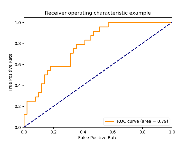
3.3.2.13. Receiver operating characteristic (ROC)
The function roc_curve computes thereceiver operating characteristic curve, or ROC curve. Quoting Wikipedia :
“A receiver operating characteristic (ROC), or simply ROC curve, is a graphical plot which illustrates the performance of a binary classifier system as its discrimination threshold is varied. It is created by plotting the fraction of true positives out of the positives (TPR = true positive rate) vs. the fraction of false positives out of the negatives (FPR = false positive rate), at various threshold settings. TPR is also known as sensitivity, and FPR is one minus the specificity or true negative rate.”
This function requires the true binary value and the target scores, which can either be probability estimates of the positive class, confidence values, or binary decisions. Here is a small example of how to use the roc_curve function:
import numpy as np from sklearn.metrics import roc_curve y = np.array([1, 1, 2, 2]) scores = np.array([0.1, 0.4, 0.35, 0.8]) fpr, tpr, thresholds = roc_curve(y, scores, pos_label=2) fpr array([0. , 0. , 0.5, 0.5, 1. ]) tpr array([0. , 0.5, 0.5, 1. , 1. ]) thresholds array([1.8 , 0.8 , 0.4 , 0.35, 0.1 ])
This figure shows an example of such an ROC curve:
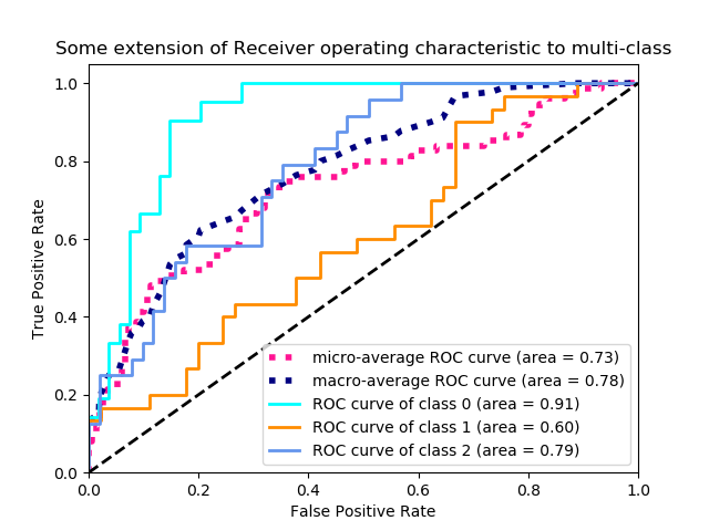
The roc_auc_score function computes the area under the receiver operating characteristic (ROC) curve, which is also denoted by AUC or AUROC. By computing the area under the roc curve, the curve information is summarized in one number. For more information see the Wikipedia article on AUC.
import numpy as np from sklearn.metrics import roc_auc_score y_true = np.array([0, 0, 1, 1]) y_scores = np.array([0.1, 0.4, 0.35, 0.8]) roc_auc_score(y_true, y_scores) 0.75
In multi-label classification, the roc_auc_score function is extended by averaging over the labels as above.
Compared to metrics such as the subset accuracy, the Hamming loss, or the F1 score, ROC doesn’t require optimizing a threshold for each label. Theroc_auc_score function can also be used in multi-class classification, if the predicted outputs have been binarized.
In applications where a high false positive rate is not tolerable the parametermax_fpr of roc_auc_score can be used to summarize the ROC curve up to the given limit.
Examples:
- See Receiver Operating Characteristic (ROC)for an example of using ROC to evaluate the quality of the output of a classifier.
- See Receiver Operating Characteristic (ROC) with cross validationfor an example of using ROC to evaluate classifier output quality, using cross-validation.
- See Species distribution modelingfor an example of using ROC to model species distribution.
3.3.2.14. Zero one loss
The zero_one_loss function computes the sum or the average of the 0-1 classification loss (\(L_{0-1}\)) over \(n_{\text{samples}}\). By default, the function normalizes over the sample. To get the sum of the\(L_{0-1}\), set normalize to False.
In multilabel classification, the zero_one_loss scores a subset as one if its labels strictly match the predictions, and as a zero if there are any errors. By default, the function returns the percentage of imperfectly predicted subsets. To get the count of such subsets instead, setnormalize to False
If \(\hat{y}_i\) is the predicted value of the \(i\)-th sample and \(y_i\) is the corresponding true value, then the 0-1 loss \(L_{0-1}\) is defined as:
\[L_{0-1}(y_i, \hat{y}_i) = 1(\hat{y}_i \not= y_i)\]
where \(1(x)\) is the indicator function.
from sklearn.metrics import zero_one_loss y_pred = [1, 2, 3, 4] y_true = [2, 2, 3, 4] zero_one_loss(y_true, y_pred) 0.25 zero_one_loss(y_true, y_pred, normalize=False) 1
In the multilabel case with binary label indicators, where the first label set [0,1] has an error:
zero_one_loss(np.array([[0, 1], [1, 1]]), np.ones((2, 2))) 0.5
zero_one_loss(np.array([[0, 1], [1, 1]]), np.ones((2, 2)), normalize=False) 1
Example:
- See Recursive feature elimination with cross-validationfor an example of zero one loss usage to perform recursive feature elimination with cross-validation.
3.3.2.15. Brier score loss
The brier_score_loss function computes theBrier scorefor binary classes. Quoting Wikipedia:
“The Brier score is a proper score function that measures the accuracy of probabilistic predictions. It is applicable to tasks in which predictions must assign probabilities to a set of mutually exclusive discrete outcomes.”
This function returns a score of the mean square difference between the actual outcome and the predicted probability of the possible outcome. The actual outcome has to be 1 or 0 (true or false), while the predicted probability of the actual outcome can be a value between 0 and 1.
The brier score loss is also between 0 to 1 and the lower the score (the mean square difference is smaller), the more accurate the prediction is. It can be thought of as a measure of the “calibration” of a set of probabilistic predictions.
\[BS = \frac{1}{N} \sum_{t=1}^{N}(f_t - o_t)^2\]
where : \(N\) is the total number of predictions, \(f_t\) is the predicted probability of the actual outcome \(o_t\).
Here is a small example of usage of this function::
import numpy as np from sklearn.metrics import brier_score_loss y_true = np.array([0, 1, 1, 0]) y_true_categorical = np.array(["spam", "ham", "ham", "spam"]) y_prob = np.array([0.1, 0.9, 0.8, 0.4]) y_pred = np.array([0, 1, 1, 0]) brier_score_loss(y_true, y_prob) 0.055 brier_score_loss(y_true, 1 - y_prob, pos_label=0) 0.055 brier_score_loss(y_true_categorical, y_prob, pos_label="ham") 0.055 brier_score_loss(y_true, y_prob > 0.5) 0.0
Example:
- See Probability calibration of classifiersfor an example of Brier score loss usage to perform probability calibration of classifiers.
3.3.3. Multilabel ranking metrics
In multilabel learning, each sample can have any number of ground truth labels associated with it. The goal is to give high scores and better rank to the ground truth labels.
3.3.3.1. Coverage error
The coverage_error function computes the average number of labels that have to be included in the final prediction such that all true labels are predicted. This is useful if you want to know how many top-scored-labels you have to predict in average without missing any true one. The best value of this metrics is thus the average number of true labels.
Note
Our implementation’s score is 1 greater than the one given in Tsoumakas et al., 2010. This extends it to handle the degenerate case in which an instance has 0 true labels.
Formally, given a binary indicator matrix of the ground truth labels\(y \in \left\{0, 1\right\}^{n_\text{samples} \times n_\text{labels}}\) and the score associated with each label\(\hat{f} \in \mathbb{R}^{n_\text{samples} \times n_\text{labels}}\), the coverage is defined as
\[coverage(y, \hat{f}) = \frac{1}{n_{\text{samples}}} \sum_{i=0}^{n_{\text{samples}} - 1} \max_{j:y_{ij} = 1} \text{rank}_{ij}\]
with \(\text{rank}_{ij} = \left|\left\{k: \hat{f}_{ik} \geq \hat{f}_{ij} \right\}\right|\). Given the rank definition, ties in y_scores are broken by giving the maximal rank that would have been assigned to all tied values.
Here is a small example of usage of this function:
import numpy as np from sklearn.metrics import coverage_error y_true = np.array([[1, 0, 0], [0, 0, 1]]) y_score = np.array([[0.75, 0.5, 1], [1, 0.2, 0.1]]) coverage_error(y_true, y_score) 2.5
3.3.3.2. Label ranking average precision
The label_ranking_average_precision_score function implements label ranking average precision (LRAP). This metric is linked to the average_precision_score function, but is based on the notion of label ranking instead of precision and recall.
Label ranking average precision (LRAP) averages over the samples the answer to the following question: for each ground truth label, what fraction of higher-ranked labels were true labels? This performance measure will be higher if you are able to give better rank to the labels associated with each sample. The obtained score is always strictly greater than 0, and the best value is 1. If there is exactly one relevant label per sample, label ranking average precision is equivalent to the mean reciprocal rank.
Formally, given a binary indicator matrix of the ground truth labels\(y \in \left\{0, 1\right\}^{n_\text{samples} \times n_\text{labels}}\)and the score associated with each label\(\hat{f} \in \mathbb{R}^{n_\text{samples} \times n_\text{labels}}\), the average precision is defined as
\[LRAP(y, \hat{f}) = \frac{1}{n_{\text{samples}}} \sum_{i=0}^{n_{\text{samples}} - 1} \frac{1}{||y_i||_0} \sum_{j:y_{ij} = 1} \frac{|\mathcal{L}_{ij}|}{\text{rank}_{ij}}\]
where\(\mathcal{L}_{ij} = \left\{k: y_{ik} = 1, \hat{f}_{ik} \geq \hat{f}_{ij} \right\}\),\(\text{rank}_{ij} = \left|\left\{k: \hat{f}_{ik} \geq \hat{f}_{ij} \right\}\right|\),\(|\cdot|\) computes the cardinality of the set (i.e., the number of elements in the set), and \(||\cdot||_0\) is the \(\ell_0\) “norm” (which computes the number of nonzero elements in a vector).
Here is a small example of usage of this function:
import numpy as np from sklearn.metrics import label_ranking_average_precision_score y_true = np.array([[1, 0, 0], [0, 0, 1]]) y_score = np.array([[0.75, 0.5, 1], [1, 0.2, 0.1]]) label_ranking_average_precision_score(y_true, y_score) 0.416...
3.3.3.3. Ranking loss
The label_ranking_loss function computes the ranking loss which averages over the samples the number of label pairs that are incorrectly ordered, i.e. true labels have a lower score than false labels, weighted by the inverse of the number of ordered pairs of false and true labels. The lowest achievable ranking loss is zero.
Formally, given a binary indicator matrix of the ground truth labels\(y \in \left\{0, 1\right\}^{n_\text{samples} \times n_\text{labels}}\) and the score associated with each label\(\hat{f} \in \mathbb{R}^{n_\text{samples} \times n_\text{labels}}\), the ranking loss is defined as
\[ranking\_loss(y, \hat{f}) = \frac{1}{n_{\text{samples}}} \sum_{i=0}^{n_{\text{samples}} - 1} \frac{1}{||y_i||_0(n_\text{labels} - ||y_i||_0)} \left|\left\{(k, l): \hat{f}_{ik} \leq \hat{f}_{il}, y_{ik} = 1, y_{il} = 0 \right\}\right|\]
where \(|\cdot|\) computes the cardinality of the set (i.e., the number of elements in the set) and \(||\cdot||_0\) is the \(\ell_0\) “norm” (which computes the number of nonzero elements in a vector).
Here is a small example of usage of this function:
import numpy as np from sklearn.metrics import label_ranking_loss y_true = np.array([[1, 0, 0], [0, 0, 1]]) y_score = np.array([[0.75, 0.5, 1], [1, 0.2, 0.1]]) label_ranking_loss(y_true, y_score) 0.75...
With the following prediction, we have perfect and minimal loss
y_score = np.array([[1.0, 0.1, 0.2], [0.1, 0.2, 0.9]]) label_ranking_loss(y_true, y_score) 0.0
References:
- Tsoumakas, G., Katakis, I., & Vlahavas, I. (2010). Mining multi-label data. In Data mining and knowledge discovery handbook (pp. 667-685). Springer US.
3.3.4. Regression metrics
The sklearn.metrics module implements several loss, score, and utility functions to measure regression performance. Some of those have been enhanced to handle the multioutput case: mean_squared_error,mean_absolute_error, explained_variance_score andr2_score.
These functions have an multioutput keyword argument which specifies the way the scores or losses for each individual target should be averaged. The default is 'uniform_average', which specifies a uniformly weighted mean over outputs. If an ndarray of shape (n_outputs,) is passed, then its entries are interpreted as weights and an according weighted average is returned. If multioutput is 'raw_values' is specified, then all unaltered individual scores or losses will be returned in an array of shape(n_outputs,).
The r2_score and explained_variance_score accept an additional value 'variance_weighted' for the multioutput parameter. This option leads to a weighting of each individual score by the variance of the corresponding target variable. This setting quantifies the globally captured unscaled variance. If the target variables are of different scale, then this score puts more importance on well explaining the higher variance variables.multioutput='variance_weighted' is the default value for r2_scorefor backward compatibility. This will be changed to uniform_average in the future.
3.3.4.1. Explained variance score
The explained_variance_score computes the explained variance regression score.
If \(\hat{y}\) is the estimated target output, \(y\) the corresponding (correct) target output, and \(Var\) is Variance, the square of the standard deviation, then the explained variance is estimated as follow:
\[explained\_{}variance(y, \hat{y}) = 1 - \frac{Var\{ y - \hat{y}\}}{Var\{y\}}\]
The best possible score is 1.0, lower values are worse.
Here is a small example of usage of the explained_variance_scorefunction:
from sklearn.metrics import explained_variance_score y_true = [3, -0.5, 2, 7] y_pred = [2.5, 0.0, 2, 8] explained_variance_score(y_true, y_pred)
0.957... y_true = [[0.5, 1], [-1, 1], [7, -6]] y_pred = [[0, 2], [-1, 2], [8, -5]] explained_variance_score(y_true, y_pred, multioutput='raw_values') ... array([0.967..., 1. ]) explained_variance_score(y_true, y_pred, multioutput=[0.3, 0.7]) ... 0.990...
3.3.4.2. Mean absolute error
The mean_absolute_error function computes mean absolute error, a risk metric corresponding to the expected value of the absolute error loss or\(l1\)-norm loss.
If \(\hat{y}_i\) is the predicted value of the \(i\)-th sample, and \(y_i\) is the corresponding true value, then the mean absolute error (MAE) estimated over \(n_{\text{samples}}\) is defined as
\[\text{MAE}(y, \hat{y}) = \frac{1}{n_{\text{samples}}} \sum_{i=0}^{n_{\text{samples}}-1} \left| y_i - \hat{y}_i \right|.\]
Here is a small example of usage of the mean_absolute_error function:
from sklearn.metrics import mean_absolute_error y_true = [3, -0.5, 2, 7] y_pred = [2.5, 0.0, 2, 8] mean_absolute_error(y_true, y_pred) 0.5 y_true = [[0.5, 1], [-1, 1], [7, -6]] y_pred = [[0, 2], [-1, 2], [8, -5]] mean_absolute_error(y_true, y_pred) 0.75 mean_absolute_error(y_true, y_pred, multioutput='raw_values') array([0.5, 1. ]) mean_absolute_error(y_true, y_pred, multioutput=[0.3, 0.7]) ... 0.85...
3.3.4.3. Mean squared error
The mean_squared_error function computes mean square error, a risk metric corresponding to the expected value of the squared (quadratic) error or loss.
If \(\hat{y}_i\) is the predicted value of the \(i\)-th sample, and \(y_i\) is the corresponding true value, then the mean squared error (MSE) estimated over \(n_{\text{samples}}\) is defined as
\[\text{MSE}(y, \hat{y}) = \frac{1}{n_\text{samples}} \sum_{i=0}^{n_\text{samples} - 1} (y_i - \hat{y}_i)^2.\]
Here is a small example of usage of the mean_squared_errorfunction:
from sklearn.metrics import mean_squared_error y_true = [3, -0.5, 2, 7] y_pred = [2.5, 0.0, 2, 8] mean_squared_error(y_true, y_pred) 0.375 y_true = [[0.5, 1], [-1, 1], [7, -6]] y_pred = [[0, 2], [-1, 2], [8, -5]] mean_squared_error(y_true, y_pred)
0.7083...
Examples:
- See Gradient Boosting regressionfor an example of mean squared error usage to evaluate gradient boosting regression.
3.3.4.4. Mean squared logarithmic error
The mean_squared_log_error function computes a risk metric corresponding to the expected value of the squared logarithmic (quadratic) error or loss.
If \(\hat{y}_i\) is the predicted value of the \(i\)-th sample, and \(y_i\) is the corresponding true value, then the mean squared logarithmic error (MSLE) estimated over \(n_{\text{samples}}\) is defined as
\[\text{MSLE}(y, \hat{y}) = \frac{1}{n_\text{samples}} \sum_{i=0}^{n_\text{samples} - 1} (\log_e (1 + y_i) - \log_e (1 + \hat{y}_i) )^2.\]
Where \(\log_e (x)\) means the natural logarithm of \(x\). This metric is best to use when targets having exponential growth, such as population counts, average sales of a commodity over a span of years etc. Note that this metric penalizes an under-predicted estimate greater than an over-predicted estimate.
Here is a small example of usage of the mean_squared_log_errorfunction:
from sklearn.metrics import mean_squared_log_error y_true = [3, 5, 2.5, 7] y_pred = [2.5, 5, 4, 8] mean_squared_log_error(y_true, y_pred)
0.039... y_true = [[0.5, 1], [1, 2], [7, 6]] y_pred = [[0.5, 2], [1, 2.5], [8, 8]] mean_squared_log_error(y_true, y_pred)
0.044...
3.3.4.6. R² score, the coefficient of determination
The r2_score function computes R², the coefficient of determination. It provides a measure of how well future samples are likely to be predicted by the model. Best possible score is 1.0 and it can be negative (because the model can be arbitrarily worse). A constant model that always predicts the expected value of y, disregarding the input features, would get a R^2 score of 0.0.
If \(\hat{y}_i\) is the predicted value of the \(i\)-th sample and \(y_i\) is the corresponding true value, then the score R² estimated over \(n_{\text{samples}}\) is defined as
\[R^2(y, \hat{y}) = 1 - \frac{\sum_{i=0}^{n_{\text{samples}} - 1} (y_i - \hat{y}_i)^2}{\sum_{i=0}^{n_\text{samples} - 1} (y_i - \bar{y})^2}\]
where \(\bar{y} = \frac{1}{n_{\text{samples}}} \sum_{i=0}^{n_{\text{samples}} - 1} y_i\).
Here is a small example of usage of the r2_score function:
from sklearn.metrics import r2_score y_true = [3, -0.5, 2, 7] y_pred = [2.5, 0.0, 2, 8] r2_score(y_true, y_pred)
0.948... y_true = [[0.5, 1], [-1, 1], [7, -6]] y_pred = [[0, 2], [-1, 2], [8, -5]] r2_score(y_true, y_pred, multioutput='variance_weighted') ... 0.938... y_true = [[0.5, 1], [-1, 1], [7, -6]] y_pred = [[0, 2], [-1, 2], [8, -5]] r2_score(y_true, y_pred, multioutput='uniform_average') ... 0.936... r2_score(y_true, y_pred, multioutput='raw_values') ... array([0.965..., 0.908...]) r2_score(y_true, y_pred, multioutput=[0.3, 0.7]) ... 0.925...
Example:
- See Lasso and Elastic Net for Sparse Signalsfor an example of R² score usage to evaluate Lasso and Elastic Net on sparse signals.
3.3.6. Dummy estimators
When doing supervised learning, a simple sanity check consists of comparing one’s estimator against simple rules of thumb. DummyClassifierimplements several such simple strategies for classification:
stratifiedgenerates random predictions by respecting the training set class distribution.most_frequentalways predicts the most frequent label in the training set.prioralways predicts the class that maximizes the class prior (likemost_frequent) andpredict_probareturns the class prior.uniformgenerates predictions uniformly at random.constantalways predicts a constant label that is provided by the user.
A major motivation of this method is F1-scoring, when the positive class is in the minority.
Note that with all these strategies, the predict method completely ignores the input data!
To illustrate DummyClassifier, first let’s create an imbalanced dataset:
from sklearn.datasets import load_iris from sklearn.model_selection import train_test_split iris = load_iris() X, y = iris.data, iris.target y[y != 1] = -1 X_train, X_test, y_train, y_test = train_test_split(X, y, random_state=0)
Next, let’s compare the accuracy of SVC and most_frequent:
from sklearn.dummy import DummyClassifier from sklearn.svm import SVC clf = SVC(kernel='linear', C=1).fit(X_train, y_train) clf.score(X_test, y_test) 0.63... clf = DummyClassifier(strategy='most_frequent', random_state=0) clf.fit(X_train, y_train) DummyClassifier(constant=None, random_state=0, strategy='most_frequent') clf.score(X_test, y_test)
0.57...
We see that SVC doesn’t do much better than a dummy classifier. Now, let’s change the kernel:
clf = SVC(gamma='scale', kernel='rbf', C=1).fit(X_train, y_train) clf.score(X_test, y_test)
0.94...
We see that the accuracy was boosted to almost 100%. A cross validation strategy is recommended for a better estimate of the accuracy, if it is not too CPU costly. For more information see the Cross-validation: evaluating estimator performancesection. Moreover if you want to optimize over the parameter space, it is highly recommended to use an appropriate methodology; see the Tuning the hyper-parameters of an estimatorsection for details.
More generally, when the accuracy of a classifier is too close to random, it probably means that something went wrong: features are not helpful, a hyperparameter is not correctly tuned, the classifier is suffering from class imbalance, etc…
DummyRegressor also implements four simple rules of thumb for regression:
meanalways predicts the mean of the training targets.medianalways predicts the median of the training targets.quantilealways predicts a user provided quantile of the training targets.constantalways predicts a constant value that is provided by the user.
In all these strategies, the predict method completely ignores the input data.