Feature agglomeration vs. univariate selection (original) (raw)
Note
Go to the endto download the full example code. or to run this example in your browser via JupyterLite or Binder
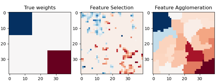
This example compares 2 dimensionality reduction strategies:
- univariate feature selection with Anova
- feature agglomeration with Ward hierarchical clustering
Both methods are compared in a regression problem using a BayesianRidge as supervised estimator.
Authors: The scikit-learn developers
SPDX-License-Identifier: BSD-3-Clause
import shutil import tempfile
import matplotlib.pyplot as plt import numpy as np from joblib import Memory from scipy import linalg, ndimage
from sklearn import feature_selection from sklearn.cluster import FeatureAgglomeration from sklearn.feature_extraction.image import grid_to_graph from sklearn.linear_model import BayesianRidge from sklearn.model_selection import GridSearchCV, KFold from sklearn.pipeline import Pipeline
Set parameters
n_samples = 200 size = 40 # image size roi_size = 15 snr = 5.0 np.random.seed(0)
Generate data
coef = np.zeros((size, size)) coef[0:roi_size, 0:roi_size] = -1.0 coef[-roi_size:, -roi_size:] = 1.0
X = np.random.randn(n_samples, size**2) for x in X: # smooth data x[:] = ndimage.gaussian_filter(x.reshape(size, size), sigma=1.0).ravel() X -= X.mean(axis=0) X /= X.std(axis=0)
y = np.dot(X, coef.ravel())
add noise
Compute the coefs of a Bayesian Ridge with GridSearch
Ward agglomeration followed by BayesianRidge
connectivity = grid_to_graph(n_x=size, n_y=size) ward = FeatureAgglomeration(n_clusters=10, connectivity=connectivity, memory=mem) clf = Pipeline([("ward", ward), ("ridge", ridge)])
Select the optimal number of parcels with grid search
clf = GridSearchCV(clf, {"ward__n_clusters": [10, 20, 30]}, n_jobs=1, cv=cv) clf.fit(X, y) # set the best parameters coef_ = clf.best_estimator_.steps[-1][1].coef_ coef_ = clf.best_estimator_.steps[0][1].inverse_transform(coef_) coef_agglomeration_ = coef_.reshape(size, size)
[Memory] Calling sklearn.cluster._agglomerative.ward_tree... ward_tree(array([[-0.451933, ..., -0.675318], ..., [ 0.275706, ..., -1.085711]], shape=(1600, 100)), connectivity=<COOrdinate sparse matrix of dtype 'int64' with 7840 stored elements and shape (1600, 1600)>, n_clusters=None, return_distance=False) ________________________________________________________ward_tree - 0.0s, 0.0min
[Memory] Calling sklearn.cluster._agglomerative.ward_tree... ward_tree(array([[ 0.905206, ..., 0.161245], ..., [-0.849835, ..., -1.091621]], shape=(1600, 100)), connectivity=<COOrdinate sparse matrix of dtype 'int64' with 7840 stored elements and shape (1600, 1600)>, n_clusters=None, return_distance=False) ________________________________________________________ward_tree - 0.0s, 0.0min
[Memory] Calling sklearn.cluster._agglomerative.ward_tree... ward_tree(array([[ 0.905206, ..., -0.675318], ..., [-0.849835, ..., -1.085711]], shape=(1600, 200)), connectivity=<COOrdinate sparse matrix of dtype 'int64' with 7840 stored elements and shape (1600, 1600)>, n_clusters=None, return_distance=False) ________________________________________________________ward_tree - 0.0s, 0.0min
Anova univariate feature selection followed by BayesianRidge
f_regression = mem.cache(feature_selection.f_regression) # caching function anova = feature_selection.SelectPercentile(f_regression) clf = Pipeline([("anova", anova), ("ridge", ridge)])
Select the optimal percentage of features with grid search
clf = GridSearchCV(clf, {"anova__percentile": [5, 10, 20]}, cv=cv) clf.fit(X, y) # set the best parameters coef_ = clf.best_estimator_.steps[-1][1].coef_ coef_ = clf.best_estimator_.steps[0][1].inverse_transform(coef_.reshape(1, -1)) coef_selection_ = coef_.reshape(size, size)
[Memory] Calling sklearn.feature_selection._univariate_selection.f_regression... f_regression(array([[-0.451933, ..., 0.275706], ..., [-0.675318, ..., -1.085711]], shape=(100, 1600)), array([ 25.267703, ..., -25.026711], shape=(100,))) _____________________________________________________f_regression - 0.0s, 0.0min
[Memory] Calling sklearn.feature_selection._univariate_selection.f_regression... f_regression(array([[ 0.905206, ..., -0.849835], ..., [ 0.161245, ..., -1.091621]], shape=(100, 1600)), array([ -27.447268, ..., -112.638768], shape=(100,))) _____________________________________________________f_regression - 0.0s, 0.0min
[Memory] Calling sklearn.feature_selection._univariate_selection.f_regression... f_regression(array([[ 0.905206, ..., -0.849835], ..., [-0.675318, ..., -1.085711]], shape=(200, 1600)), array([-27.447268, ..., -25.026711], shape=(200,))) _____________________________________________________f_regression - 0.0s, 0.0min
Inverse the transformation to plot the results on an image
plt.close("all") plt.figure(figsize=(7.3, 2.7)) plt.subplot(1, 3, 1) plt.imshow(coef, interpolation="nearest", cmap=plt.cm.RdBu_r) plt.title("True weights") plt.subplot(1, 3, 2) plt.imshow(coef_selection_, interpolation="nearest", cmap=plt.cm.RdBu_r) plt.title("Feature Selection") plt.subplot(1, 3, 3) plt.imshow(coef_agglomeration_, interpolation="nearest", cmap=plt.cm.RdBu_r) plt.title("Feature Agglomeration") plt.subplots_adjust(0.04, 0.0, 0.98, 0.94, 0.16, 0.26) plt.show()
Attempt to remove the temporary cachedir, but don’t worry if it fails
Total running time of the script: (0 minutes 0.462 seconds)
Related examples