Chapter 2 Linear models | Omics Data Analysis (original) (raw)
library("tidyverse")
## Prepare the data
x <-
    data.frame(lmdata) |>
    rownames_to_column() |>
    pivot_longer(names_to = "sample", values_to = "expression", -rowname) |>
    full_join(lmannot) |>
    mutate(sample = sub("sample_", "", sample))
## Analyse gene 1
x_i <- filter(x, rowname == "gene_1")
x_i
## # A tibble: 12 × 5
##    rowname sample expression condition cell_type
##    <chr>   <chr>       <dbl> <chr>     <chr>
##  1 gene_1  1            4.44 ctrl      A
##  2 gene_1  2            4.77 ctrl      B
##  3 gene_1  3            6.56 ctrl      A
##  4 gene_1  4            5.07 ctrl      B
##  5 gene_1  5            5.13 ctrl      A
##  6 gene_1  6            6.72 ctrl      B
##  7 gene_1  7            5.46 cond      A
##  8 gene_1  8            3.73 cond      B
##  9 gene_1  9            4.31 cond      A
## 10 gene_1  10           4.55 cond      B
## 11 gene_1  11           6.22 cond      A
## 12 gene_1  12           5.36 cond      B
mod_i <- lm(expression ~ condition * cell_type, data = x_i)
summary(mod_i)
##
## Call:
## lm(formula = expression ~ condition * cell_type, data = x_i)
##
## Residuals:
##     Min      1Q  Median      3Q     Max
## -1.0196 -0.7652 -0.1210  0.8304  1.1966
##
## Coefficients:
##                          Estimate Std. Error t value Pr(>|t|)
## (Intercept)               5.33272    0.56643   9.415 1.33e-05 ***
## conditionctrl             0.04312    0.80105   0.054    0.958
## cell_typeB               -0.78302    0.80105  -0.977    0.357
## conditionctrl:cell_typeB  0.92564    1.13286   0.817    0.438
## ---
## Signif. codes:  0 '***' 0.001 '**' 0.01 '*' 0.05 '.' 0.1 ' ' 1
##
## Residual standard error: 0.9811 on 8 degrees of freedom
## Multiple R-squared:  0.1824, Adjusted R-squared:  -0.1242
## F-statistic: 0.595 on 3 and 8 DF,  p-value: 0.6357
ggplot(x_i, aes(x = sample, y = expression,
                colour = condition,
                shape = cell_type)) +
    geom_point()
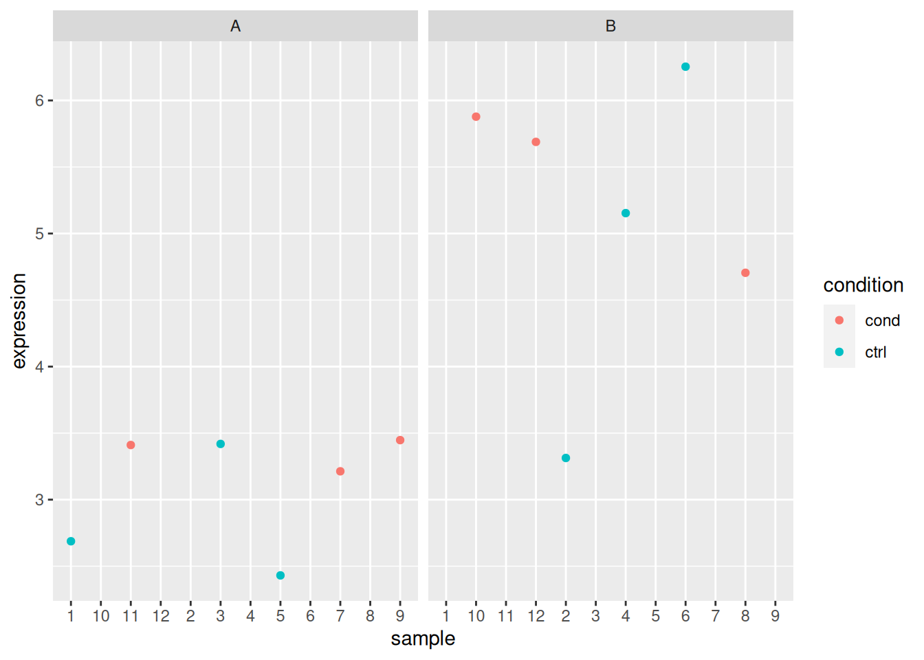
## Analyse gene 2
x_i <- filter(x, rowname == "gene_2")
x_i
## # A tibble: 12 × 5
##    rowname sample expression condition cell_type
##    <chr>   <chr>       <dbl> <chr>     <chr>
##  1 gene_2  1            6.16 ctrl      A
##  2 gene_2  2            6.04 ctrl      B
##  3 gene_2  3            5.78 ctrl      A
##  4 gene_2  4            6.71 ctrl      B
##  5 gene_2  5            6.20 ctrl      A
##  6 gene_2  6            5.21 ctrl      B
##  7 gene_2  7            4.70 cond      A
##  8 gene_2  8            3.53 cond      B
##  9 gene_2  9            2.93 cond      A
## 10 gene_2  10           3.78 cond      B
## 11 gene_2  11           2.97 cond      A
## 12 gene_2  12           3.27 cond      B
mod_i <- lm(expression ~ condition * cell_type, data = x_i)
summary(mod_i)
##
## Call:
## lm(formula = expression ~ condition * cell_type, data = x_i)
##
## Residuals:
##      Min       1Q   Median       3Q      Max
## -0.77745 -0.34149  0.02695  0.17889  1.16551
##
## Coefficients:
##                           Estimate Std. Error t value Pr(>|t|)
## (Intercept)               3.535847   0.376883   9.382 1.36e-05 ***
## conditionctrl             2.509857   0.532992   4.709  0.00152 **
## cell_typeB               -0.009063   0.532992  -0.017  0.98685
## conditionctrl:cell_typeB -0.045843   0.753765  -0.061  0.95300
## ---
## Signif. codes:  0 '***' 0.001 '**' 0.01 '*' 0.05 '.' 0.1 ' ' 1
##
## Residual standard error: 0.6528 on 8 degrees of freedom
## Multiple R-squared:  0.8448, Adjusted R-squared:  0.7866
## F-statistic: 14.52 on 3 and 8 DF,  p-value: 0.001335
ggplot(x_i, aes(x = sample, y = expression, colour = cell_type)) +
    geom_point() +
    facet_wrap(~ condition)
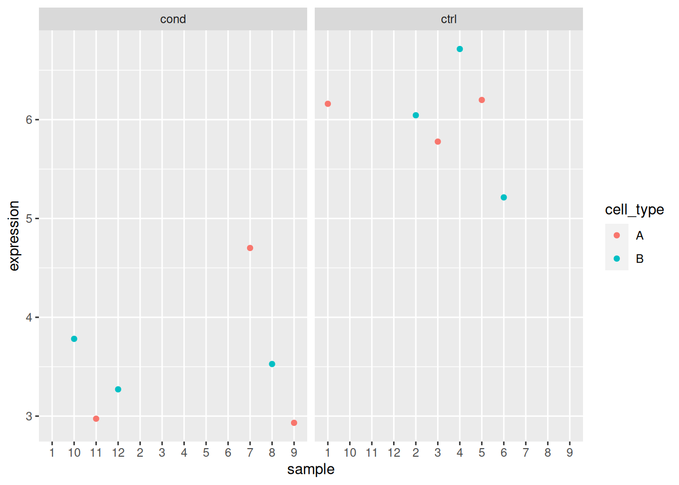
## Analyse gene 3
x_i <- filter(x, rowname == "gene_3")
x_i
## # A tibble: 12 × 5
##    rowname sample expression condition cell_type
##    <chr>   <chr>       <dbl> <chr>     <chr>
##  1 gene_3  1            2.69 ctrl      A
##  2 gene_3  2            3.31 ctrl      B
##  3 gene_3  3            3.42 ctrl      A
##  4 gene_3  4            5.15 ctrl      B
##  5 gene_3  5            2.43 ctrl      A
##  6 gene_3  6            6.25 ctrl      B
##  7 gene_3  7            3.21 cond      A
##  8 gene_3  8            4.70 cond      B
##  9 gene_3  9            3.45 cond      A
## 10 gene_3  10           5.88 cond      B
## 11 gene_3  11           3.41 cond      A
## 12 gene_3  12           5.69 cond      B
mod_i <- lm(expression ~ condition * cell_type, data = x_i)
summary(mod_i)
##
## Call:
## lm(formula = expression ~ condition * cell_type, data = x_i)
##
## Residuals:
##      Min       1Q   Median       3Q      Max
## -1.59352 -0.22242  0.07198  0.31211  1.34698
##
## Coefficients:
##                           Estimate Std. Error t value Pr(>|t|)
## (Intercept)               3.357193   0.490117   6.850 0.000131 ***
## conditionctrl            -0.511427   0.693130  -0.738 0.481685
## cell_typeB                2.066707   0.693130   2.982 0.017555 *
## conditionctrl:cell_typeB -0.005643   0.980234  -0.006 0.995547
## ---
## Signif. codes:  0 '***' 0.001 '**' 0.01 '*' 0.05 '.' 0.1 ' ' 1
##
## Residual standard error: 0.8489 on 8 degrees of freedom
## Multiple R-squared:  0.7019, Adjusted R-squared:  0.5901
## F-statistic: 6.278 on 3 and 8 DF,  p-value: 0.01696
ggplot(x_i, aes(x = sample, y = expression, colour = condition)) +
    geom_point() +
    facet_wrap(~ cell_type)
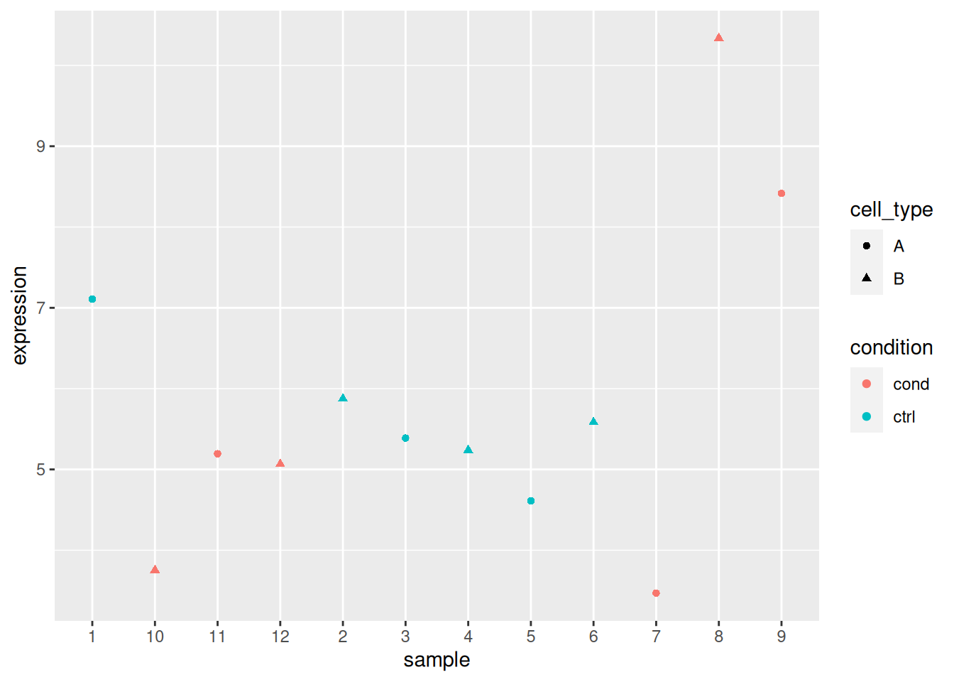
## Analyse gene 4
x_i <- filter(x, rowname == "gene_4")
x_i
## # A tibble: 12 × 5
##    rowname sample expression condition cell_type
##    <chr>   <chr>       <dbl> <chr>     <chr>
##  1 gene_4  1            7.11 ctrl      A
##  2 gene_4  2            5.88 ctrl      B
##  3 gene_4  3            5.39 ctrl      A
##  4 gene_4  4            5.24 ctrl      B
##  5 gene_4  5            4.61 ctrl      A
##  6 gene_4  6            5.58 ctrl      B
##  7 gene_4  7            3.47 cond      A
##  8 gene_4  8           10.3  cond      B
##  9 gene_4  9            8.42 cond      A
## 10 gene_4  10           3.75 cond      B
## 11 gene_4  11           5.19 cond      A
## 12 gene_4  12           5.07 cond      B
mod_i <- lm(expression ~ condition * cell_type, data = x_i)
summary(mod_i)
##
## Call:
## lm(formula = expression ~ condition * cell_type, data = x_i)
##
## Residuals:
##     Min      1Q  Median      3Q     Max
## -2.6323 -1.1485 -0.3208  0.5837  3.9518
##
## Coefficients:
##                           Estimate Std. Error t value Pr(>|t|)
## (Intercept)               5.693120   1.296865   4.390  0.00232 **
## conditionctrl             0.009047   1.834044   0.005  0.99619
## cell_typeB                0.693007   1.834044   0.378  0.71537
## conditionctrl:cell_typeB -0.828703   2.593730  -0.320  0.75753
## ---
## Signif. codes:  0 '***' 0.001 '**' 0.01 '*' 0.05 '.' 0.1 ' ' 1
##
## Residual standard error: 2.246 on 8 degrees of freedom
## Multiple R-squared:  0.02982,    Adjusted R-squared:  -0.334
## F-statistic: 0.08197 on 3 and 8 DF,  p-value: 0.968
ggplot(x_i, aes(x = sample, y = expression,
                colour = condition,
                shape = cell_type)) +
    geom_point()
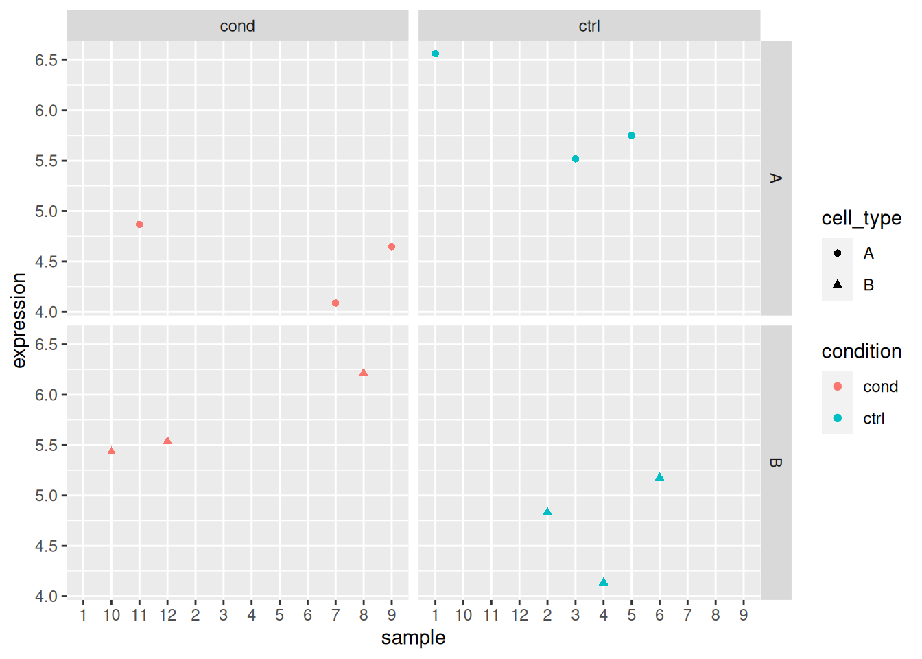
## Analyse gene 5
x_i <- filter(x, rowname == "gene_5")
x_i
## # A tibble: 12 × 5
##    rowname sample expression condition cell_type
##    <chr>   <chr>       <dbl> <chr>     <chr>
##  1 gene_5  1            6.56 ctrl      A
##  2 gene_5  2            4.83 ctrl      B
##  3 gene_5  3            5.52 ctrl      A
##  4 gene_5  4            4.14 ctrl      B
##  5 gene_5  5            5.75 ctrl      A
##  6 gene_5  6            5.18 ctrl      B
##  7 gene_5  7            4.09 cond      A
##  8 gene_5  8            6.21 cond      B
##  9 gene_5  9            4.65 cond      A
## 10 gene_5  10           5.43 cond      B
## 11 gene_5  11           4.87 cond      A
## 12 gene_5  12           5.54 cond      B
mod_i <- lm(expression ~ condition * cell_type, data = x_i)
summary(mod_i)
##
## Call:
## lm(formula = expression ~ condition * cell_type, data = x_i)
##
## Residuals:
##      Min       1Q   Median       3Q      Max
## -0.57907 -0.32745 -0.03921  0.36578  0.61935
##
## Coefficients:
##                          Estimate Std. Error t value Pr(>|t|)
## (Intercept)                4.5338     0.2775  16.338 1.98e-07 ***
## conditionctrl              1.4092     0.3924   3.591  0.00708 **
## cell_typeB                 1.1929     0.3924   3.040  0.01607 *
## conditionctrl:cell_typeB  -2.4201     0.5550  -4.361  0.00241 **
## ---
## Signif. codes:  0 '***' 0.001 '**' 0.01 '*' 0.05 '.' 0.1 ' ' 1
##
## Residual standard error: 0.4806 on 8 degrees of freedom
## Multiple R-squared:  0.7094, Adjusted R-squared:  0.6005
## F-statistic: 6.511 on 3 and 8 DF,  p-value: 0.01536
group_by(x_i, cell_type, condition) |> summarise(mean = mean(expression))
## `summarise()` has grouped output by 'cell_type'. You can override using the
## `.groups` argument.
## # A tibble: 4 × 3
## # Groups:   cell_type [2]
##   cell_type condition  mean
##   <chr>     <chr>     <dbl>
## 1 A         cond       4.53
## 2 A         ctrl       5.94
## 3 B         cond       5.73
## 4 B         ctrl       4.72
group_by(x_i, cell_type) |> summarise(mean = mean(expression))
## # A tibble: 2 × 2
##   cell_type  mean
##   <chr>     <dbl>
## 1 A          5.24
## 2 B          5.22
group_by(x_i, condition) |> summarise(mean = mean(expression))
## # A tibble: 2 × 2
##   condition  mean
##   <chr>     <dbl>
## 1 cond       5.13
## 2 ctrl       5.33
ggplot(x_i, aes(x = sample, y = expression,
                colour = condition,
                shape = cell_type)) +
    geom_point() +
    facet_grid(cell_type ~ condition)