Create and Train Network with Nested Layers - MATLAB & Simulink (original) (raw)

This example shows how to create and train a network with nested layers using network layers.

There are two ways to created nested layers:

Create a networkLayer object that contains a nested network. The network layer is a single layer that behaves identically to the nested network during training and inference. You can use network layers to simplify building and editing large networks or networks with repeating components.
Create a custom layer that itself defines a neural network by specifying a dlnetwork object as a learnable parameter. This method is known as network composition and you can use network composition to create a network with control flow, for example, a network with a section that can dynamically change depending on the input data, create a network with loops, for example, a network with sections that feed the output back into itself, and implement weight sharing, for example, in networks where different data needs to pass through the same layers such as twin neural networks or generative adversarial networks (GANs). For more information, see Deep Learning Network Composition.

This example shows how to train a network using network layers containing residual blocks, each containing multiple convolution, batch normalization, and ReLU layers with a skip connection. For an example showing how to create a residual network using network composition, see Train Network with Custom Nested Layers. For this use case, it's typically easier to use the resnetNetwork function. For an example showing how to create a residual network using resnetNetwork, see Train Residual Network for Image Classification.

Residual connections are a popular element in convolutional neural network architectures. A residual network is a type of network that has residual (or shortcut) connections that bypass the main network layers. Using residual connections improves gradient flow through the network and enables the training of deeper networks. This increased network depth can yield higher accuracy on more difficult tasks.

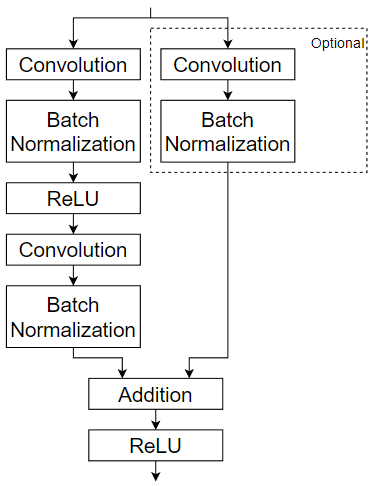
This example creates network layers each containing convolution, batch normalization, ReLU, and addition layers, and also including a skip connection and an optional convolution layer and batch normalization layer in the skip connection. This diagram highlights the residual block structure.

Prepare Data

Download and extract the Flowers data set [1].

url = "http://download.tensorflow.org/example_images/flower_photos.tgz"; downloadFolder = tempdir; filename = fullfile(downloadFolder,"flower_dataset.tgz");

imageFolder = fullfile(downloadFolder,"flower_photos"); if ~exist(imageFolder,"dir") disp("Downloading Flowers data set (218 MB)... ") websave(filename,url); untar(filename,downloadFolder) disp("Done.") end

Downloading Flowers data set (218 MB)...

Create an image datastore containing the photos.

datasetFolder = fullfile(imageFolder); imds = imageDatastore(datasetFolder, ... IncludeSubfolders=true, ... LabelSource="foldernames");

Partition the data into training and validation data sets. Use 70% of the images for training and 30% for validation.

[imdsTrain,imdsValidation] = splitEachLabel(imds,0.7,"randomized");

View the number of classes of the data set.

classes = categories(imds.Labels); numClasses = numel(classes)

Data augmentation helps prevent the network from overfitting and memorizing the exact details of the training images. Resize and augment the images for training using an imageDataAugmenter object:

Randomly reflect the images in the vertical axis.
Randomly translate the images up to 30 pixels vertically and horizontally.
Randomly rotate the images up to 45 degrees clockwise and counterclockwise.
Randomly scale the images up to 10% vertically and horizontally.

pixelRange = [-30 30]; scaleRange = [0.9 1.1]; imageAugmenter = imageDataAugmenter( ... RandXReflection=true, ... RandXTranslation=pixelRange, ... RandYTranslation=pixelRange, ... RandRotation=[-45 45], ... RandXScale=scaleRange, ... RandYScale=scaleRange);

Create an augmented image datastore containing the training data using the image data augmenter. To automatically resize the images to the network input size, specify the height and width of the input size of the network. This example uses a network with input size [224 224 3].

inputSize = [224 224 3]; augimdsTrain = augmentedImageDatastore(inputSize(1:2),imdsTrain,DataAugmentation=imageAugmenter);

To automatically resize the validation images without performing further data augmentation, use an augmented image datastore without specifying any additional preprocessing operations.

augimdsValidation = augmentedImageDatastore([224 224],imdsValidation);

Define Network Architecture

The residualBlockLayer function returns a network layer containing a residual block with an optional convolution operation in the skip connection. The numFilters and stride arguments define the number of filters and stride of the convolution layers respectively, The includeSkipConvolution argument specifies whether the skip connection includes a convolution and batch normalization layer. The name argument specifies the name of the network layer.

function layer = residualBlockLayer(numFilters,stride,includeSkipConvolution,name)

% Create empty dlnetwork. net = dlnetwork;

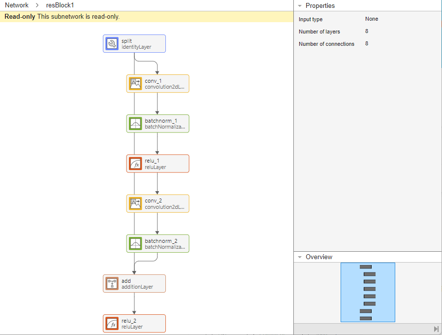
% Specify layers in the main branch and add them to the network. layers = [ functionLayer(@(X) X,Formattable=true,Acceleratable=true,Name="split") convolution2dLayer(3,numFilters,Padding="same",Stride=stride) batchNormalizationLayer reluLayer convolution2dLayer(3,numFilters,Padding="same") batchNormalizationLayer additionLayer(2,Name="add") reluLayer]; net = addLayers(net,layers);

if includeSkipConvolution % Add convolution and batch normalization layers to the skip % connection. skipLayers = [ convolution2dLayer(1,numFilters,Stride=stride,Name="skipConv") batchNormalizationLayer(Name="bnSkip")]; net = addLayers(net,skipLayers);

% Connect the layers in the skip connection.
net = connectLayers(net,"split","skipConv");
net = connectLayers(net,"bnSkip","add/in2");

else net = connectLayers(net,"split","add/in2"); end

% Create network layer containing residual block. layer = networkLayer(net,Name=name);

end

Define a residual network with six residual blocks using the residualBlockLayer function.

numFilters = 32;

layers = [ imageInputLayer(inputSize) convolution2dLayer(7,numFilters,Stride=2,Padding="same") batchNormalizationLayer reluLayer maxPooling2dLayer(3,Stride=2) residualBlockLayer(numFilters,1,false,"resBlock1") residualBlockLayer(numFilters,1,false,"resBlock2") residualBlockLayer(2numFilters,2,true,"resBlock3") residualBlockLayer(2numFilters,1,false,"resBlock4") residualBlockLayer(4numFilters,2,true,"resBlock5") residualBlockLayer(4numFilters,1,false,"resBlock6") globalAveragePooling2dLayer fullyConnectedLayer(numClasses) softmaxLayer];

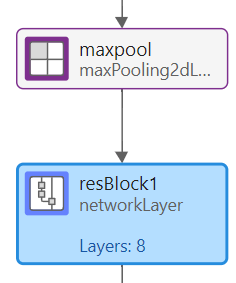
Inspect the network. To view all of the layers in the residual blocks, you can use the expandLayers function. To regroup layers back into network layers, use the groupLayers function.

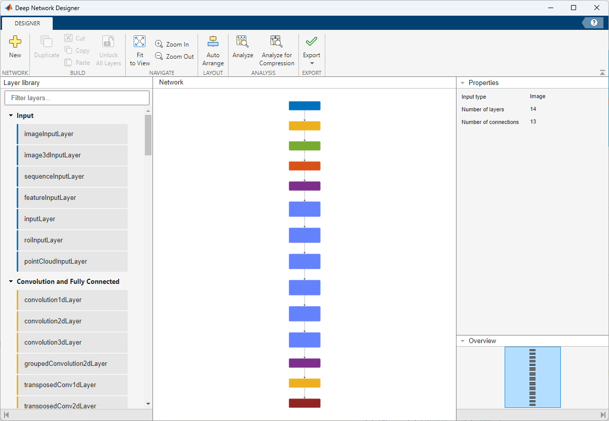
To visualize and edit layers in a network layer using Deep Network Designer, you can expand the network using the expandLayers function before opening the network in Deep Network Designer. After editing the network and exporting it to the workspace, you can regroup the layers into network layers using the groupLayers function. Adding a network layer to a network in Deep Network Designer is not supported.

Train Network

Specify training options:

Train the network with a mini-batch size of 128.
Shuffle the data every epoch.
Validate the network once per epoch using the validation data.
Output the network with lowest validation loss.
Display the training progress in a plot and monitor the accuracy.
Disable the verbose output.

miniBatchSize = 128; numIterationsPerEpoch = floor(augimdsTrain.NumObservations/miniBatchSize);

options = trainingOptions("adam", ... MiniBatchSize=miniBatchSize, ... Shuffle="every-epoch", ... ValidationData=augimdsValidation, ... ValidationFrequency=numIterationsPerEpoch, ... OutputNetwork="best-validation", ... Plots="training-progress", ... Metrics="accuracy",... Verbose=false);

Train the neural network using the trainnet function. For classification, use cross-entropy loss. By default, the trainnet function uses a GPU if one is available. Training on a GPU requires a Parallel Computing Toolbox™ license and a supported GPU device. For information on supported devices, see GPU Computing Requirements (Parallel Computing Toolbox). Otherwise, the trainnet function uses the CPU. To specify the execution environment, use the ExecutionEnvironment training option.

net = trainnet(augimdsTrain,layers,"crossentropy",options);

Evaluate Trained Network

Classify the test images. To make predictions with multiple observations, use the minibatchpredict function. To covert the prediction scores to labels, use the scores2label function. The minibatchpredict function automatically uses a GPU if one is available.

scores = minibatchpredict(net,augimdsValidation); YPred = scores2label(scores,classes);

Calculate the final accuracy of the network on the training set (without data augmentation) and validation set. The accuracy is the proportion of images that the network classifies correctly.

YValidation = imdsValidation.Labels; accuracy = mean(YPred == YValidation)

Visualize the classification accuracy in a confusion matrix. Display the precision and recall for each class by using column and row summaries.

figure confusionchart(YValidation,YPred, ... RowSummary="row-normalized", ... ColumnSummary="column-normalized");

You can display four sample validation images with predicted labels and the predicted probabilities of the images having those labels using the following code.

idx = randperm(numel(imdsValidation.Files),4); figure for i = 1:4 subplot(2,2,i) I = readimage(imdsValidation,idx(i)); imshow(I) label = YPred(idx(i)); title("Predicted class: " + string(label)); end

References

The TensorFlow Team. Flowers http://download.tensorflow.org/example_images/flower_photos.tgz