Custom Training with Multiple GPUs in Experiment Manager - MATLAB & Simulink (original) (raw)
Main Content
This example shows how to configure multiple parallel workers to collaborate on each trial of a custom training experiment. In this example, parallel workers train on portions of the overall mini-batch in each trial of an image classification experiment. During training, a DataQueue object sends training progress information back to Experiment Manager. If you have a supported GPU, then training happens on the GPU. For more information, see GPU Computing Requirements (Parallel Computing Toolbox).
As an alternative, you can set up a parallel custom training loop that runs a single trial of this experiment programmatically. For more information, see Train Network in Parallel with Custom Training Loop.
Open Experiment
First, open the example. Experiment Manager loads a project with a preconfigured experiment that you can inspect and run. To open the experiment, in the Experiment Browser pane, double-click ParallelCustomLoopExperiment.
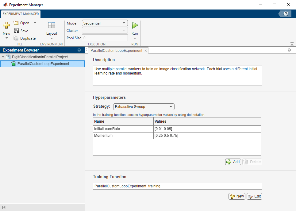
Custom training experiments consist of a description, a table of hyperparameters, and a training function. For more information, see Train Network Using Custom Training Loop and Display Visualization.
The Description field contains a textual description of the experiment. For this example, the description is:
Use multiple parallel workers to train an image classification network. Each trial uses a different initial learning rate and momentum.
The Hyperparameters section specifies the strategy and hyperparameter values to use for the experiment. When you run the experiment, Experiment Manager trains the network using every combination of hyperparameter values specified in the hyperparameter table. This example uses two hyperparameters:
InitialLearnRatesets the initial learning rate used for training. If the learning rate is too low, then training takes a long time. If the learning rate is too high, then training can reach a suboptimal result or diverge. The best learning rate depends on your data as well as the network you are training.Momentumspecifies the contribution of the gradient step from the previous iteration to the current iteration of stochastic gradient descent with momentum.
The Training Function section specifies a function that defines the training data, network architecture, training options, and training procedure used by the experiment. To open this function in MATLAB® Editor, click Edit. The code for the function also appears in Training Function. The input to the training function is a structure with fields from the hyperparameter table and an experiments.Monitor object that you can use to track the progress of the training, record values of the metrics used by the training, and produce training plots. The function returns a structure that contains the trained network, the training loss, and the validation accuracy. Experiment Manager saves this output so you can export it to the MATLAB workspace when the training is complete. The training function has these sections:
- Initialize Output sets the initial value of the network, training loss, and validation accuracy to empty arrays to indicate that the training has not started.
output.network = []; output.loss = []; output.accuracy = [];
- Load Training and Test Data defines the training and test data for the experiment as
imageDatastoreobjects. The experiment uses the Digits data set, which consists of 5000 28-by-28 pixel grayscale images of digits from 0 to 9, categorized by the digit they represent. For more information on this data set, see Image Data Sets.
monitor.Status = "Loading Data";
dataFolder = fullfile(toolboxdir('nnet'), ... 'nndemos','nndatasets','DigitDataset'); imds = imageDatastore(dataFolder, ... IncludeSubfolders=true, ... LabelSource="foldernames"); [imdsTrain,imdsTest] = splitEachLabel(imds,0.9,"randomized");
classes = categories(imdsTrain.Labels); numClasses = numel(classes);
XTest = readall(imdsTest); XTest = cat(4,XTest{:}); XTest = single(XTest) ./ 255; trueLabels = imdsTest.Labels;
- Define Network Architecture defines the architecture for the image classification network. This network architecture includes batch normalization layers that track the mean and variance statistics of the data set. When training in parallel, to ensure the network state reflects the whole mini-batch, combine the statistics from all of the workers at the end of each iteration step. Otherwise, the network state can diverge across the workers. If you are training stateful recurrent neural networks (RNNs), for example, using sequence data that has been split into smaller sequences to train networks containing LSTM or GRU layers, you must also manage the state between the workers. To train the network with a custom training loop and enable automatic differentiation, the training function converts the layer graph to a dlnetwork object.
monitor.Status = "Creating Network";
layers = [ imageInputLayer([28 28 1],Normalization="none") convolution2dLayer(5,20) batchNormalizationLayer reluLayer convolution2dLayer(3,20,Padding=1) batchNormalizationLayer reluLayer convolution2dLayer(3,20,Padding=1) batchNormalizationLayer reluLayer fullyConnectedLayer(numClasses)];
lgraph = layerGraph(layers);
net = dlnetwork(lgraph);
- Set Up Parallel Environment determines if GPUs are available for MATLAB to use. If there are GPUs available, then train on the GPUs. If no parallel pool exists, create one with as many workers as GPUs. If there are no GPUs available, then train on the CPUs. If no parallel pool exists, create one with the default number of workers.
monitor.Status = "Starting Parallel Pool";
pool = gcp("nocreate");
if canUseGPU executionEnvironment = "gpu"; if isempty(pool) numberOfGPUs = gpuDeviceCount("available"); pool = parpool(numberOfGPUs); end else executionEnvironment = "cpu"; if isempty(pool) pool = parpool; end end
N = pool.NumWorkers;
- Specify Training Options defines the training options used by the experiment. In this example, Experiment Manager trains the network with a mini-batch size of
128for20epochs using the initial learning rate and momentum defined in the hyperparameter table. If you are training on a GPU, the mini-batch size scales up linearly with the number of GPUs to keep the workload on each GPU constant. For more information, see Deep Learning with MATLAB on Multiple GPUs.
numEpochs = 20; miniBatchSize = 128; velocity = []; initialLearnRate = params.InitialLearnRate; momentum = params.Momentum; decay = 0.01;
if executionEnvironment == "gpu" miniBatchSize = miniBatchSize .* N; end
workerMiniBatchSize = floor(miniBatchSize ./ repmat(N,1,N)); remainder = miniBatchSize - sum(workerMiniBatchSize); workerMiniBatchSize = workerMiniBatchSize + [ones(1,remainder) zeros(1,N-remainder)];
- Train Model defines the parallel custom training loop used by the experiment. To execute the code simultaneously on all the workers, the training function uses an
spmdblock that cannot containbreak,continue, orreturnstatements. As a result, you cannot interrupt a trial of the experiment while training is in progress. If you press Stop, Experiment Manager runs the current trial to completion before stopping the experiment. For more information on the parallel custom training loop, see Appendix 1 at the end of this example.
monitor.Metrics = ["TrainingLoss" "ValidationAccuracy"]; monitor.XLabel = "Iteration"; monitor.Status = "Training";
Q = parallel.pool.DataQueue; updateFcn = @(x) updateTrainingProgress(x,monitor); afterEach(Q,updateFcn);
spmd workerImds = partition(imdsTrain,N,spmdIndex); workerImds.ReadSize = workerMiniBatchSize(spmdIndex);
workerVelocity = velocity;

iteration = 0;
lossArray = [];
accuracyArray = [];

for epoch = 1:numEpochs
    reset(workerImds);
    workerImds = shuffle(workerImds);

    if ~monitor.Stop
        while spmdReduce(@and,hasdata(workerImds))
            iteration = iteration + 1;

            [workerXBatch,workerTBatch] = read(workerImds);
            workerXBatch = cat(4,workerXBatch{:});
            workerNumObservations = numel(workerTBatch.Label);

            workerXBatch =  single(workerXBatch) ./ 255;

            workerY = zeros(numClasses,workerNumObservations,"single");
            for c = 1:numClasses
                workerY(c,workerTBatch.Label==classes(c)) = 1;
            end

            workerX = dlarray(workerXBatch,"SSCB");

            if executionEnvironment == "gpu"
                workerX = gpuArray(workerX);
            end

            [workerLoss,workerGradients,workerState] = dlfeval(@modelLoss,net,workerX,workerY);

            workerNormalizationFactor = workerMiniBatchSize(spmdIndex)./miniBatchSize;
            loss = spmdPlus(workerNormalizationFactor*extractdata(workerLoss));

            net.State = aggregateState(workerState,workerNormalizationFactor);

            workerGradients.Value = dlupdate(@aggregateGradients,workerGradients.Value,{workerNormalizationFactor});

            learnRate = initialLearnRate/(1 + decay*iteration);

            [net.Learnables,workerVelocity] = sgdmupdate(net.Learnables,workerGradients,workerVelocity,learnRate,momentum);
        end

        if spmdIndex == 1
            YPredScores = predict(net,dlarray(XTest,"SSCB"));
            [~,idx] = max(YPredScores,[],1);
            Ypred = classes(idx);
            accuracy = mean(Ypred==trueLabels);

            lossArray = [lossArray; iteration, loss];
            accuracyArray = [accuracyArray; iteration, accuracy];

            data = [numEpochs epoch iteration loss accuracy];
            send(Q,gather(data));
        end
    end
end
end
output.network = net{1}; output.loss = lossArray{1}; output.accuracy = accuracyArray{1}; predictedLabels = categorical(Ypred{1});
delete(gcp("nocreate"));
- Plot Confusion Matrix calls the confusionchart function to create the confusion matrix for the validation data. When the training is complete, the Review Results gallery in the toolstrip displays a button for the confusion matrix. The
Nameproperty of the figure specifies the name of the button. You can click the button to display the confusion matrix in the Visualizations pane.
figure(Name="Confusion Matrix") confusionchart(trueLabels,predictedLabels, ... ColumnSummary="column-normalized", ... RowSummary="row-normalized", ... Title="Confusion Matrix for Validation Data");
Run Experiment
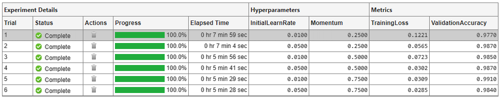
When you run the experiment, Experiment Manager trains the network defined by the training function multiple times. Each trial uses a different combination of hyperparameter values.
Because this experiment uses the parallel pool for this MATLAB session, you cannot train multiple trials at the same time. On the Experiment Manager toolstrip, set Mode to Sequential and click Run. Alternatively, to offload the experiment as a batch job, set Mode to Batch Sequential, specify your Cluster and Pool Size, and click Run. For more information, see Offload Experiments as Batch Jobs to a Cluster.
A table of results displays the training loss and validation accuracy for each trial.
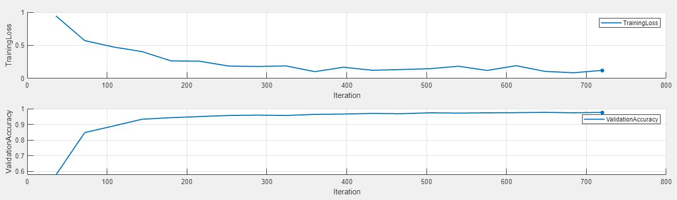
To display the training plot and track the progress of each trial while the experiment is running, under Review Results, click Training Plot.
Note that the training function for this experiment uses an spmd statement, which cannot contain break, continue, or return statements. As a result, you cannot interrupt a trial of the experiment while training is in progress. If you click Stop, Experiment Manager runs the current trial to completion before stopping the experiment.
Evaluate Results
To find the best result for your experiment, sort the table of results by validation accuracy:
- Point to the ValidationAccuracy column.
- Click the triangle icon.
- Select Sort in Descending Order.
The trial with the highest validation accuracy appears at the top of the results table.

To display the confusion matrix for this trial, select the top row in the results table and, under Review Results, click Confusion Matrix.

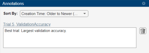
To record observations about the results of your experiment, add an annotation:
- In the results table, right-click the ValidationAccuracy cell of the best trial.
- Select Add Annotation.
- In the Annotations pane, enter your observations in the text box.
Close Experiment
In the Experiment Browser pane, right-click DigitClassificationInParallelProject and select Close Project. Experiment Manager closes the experiment and results contained in the project.
Training Function
This function configures the training data, network architecture, and training options for the experiment. To execute the code simultaneously on all the workers, the function uses an spmd block. Within the spmd block, spmdIndex gives the index of the worker currently executing the code. Before training, the function partitions the datastore for each worker by using the partition function, and sets ReadSize to the mini-batch size of the worker. For each epoch, the function resets and shuffles the datastore. For each iteration in the epoch, the function:
- Reads a mini-batch from the datastore and process the data for training.
- Computes the loss and the gradients of the network on each worker by calling
dlfevalon themodelLossfunction. - Obtains the overall loss using cross-entropy and aggregates the losses on all workers using the sum of all losses.
- Aggregates and updates the gradients of all workers using the
dlupdatefunction with theaggregateGradientsfunction. - Aggregates the state of the network on all workers using the
aggregateStatefunction. - Updates the network learnable parameters with the
sgdmupdatefunction.
At the end of each epoch, the function uses only worker to send the training progress information back to the client.
function output = ParallelCustomLoopExperiment_training(params,monitor)
Initialize Output
output.network = []; output.loss = []; output.accuracy = [];
Load Training and Test Data
monitor.Status = "Loading Data";
dataFolder = fullfile(toolboxdir('nnet'), ... 'nndemos','nndatasets','DigitDataset'); imds = imageDatastore(dataFolder, ... IncludeSubfolders=true, ... LabelSource="foldernames"); [imdsTrain,imdsTest] = splitEachLabel(imds,0.9,"randomized");
classes = categories(imdsTrain.Labels); numClasses = numel(classes);
XTest = readall(imdsTest); XTest = cat(4,XTest{:}); XTest = single(XTest) ./ 255; trueLabels = imdsTest.Labels;
Define Network Architecture
monitor.Status = "Creating Network";
layers = [ imageInputLayer([28 28 1],Normalization="none") convolution2dLayer(5,20) batchNormalizationLayer reluLayer convolution2dLayer(3,20,Padding=1) batchNormalizationLayer reluLayer convolution2dLayer(3,20,Padding=1) batchNormalizationLayer reluLayer fullyConnectedLayer(numClasses)];
lgraph = layerGraph(layers);
net = dlnetwork(lgraph);
Set Up Parallel Environment
monitor.Status = "Starting Parallel Pool";
pool = gcp("nocreate");
if canUseGPU executionEnvironment = "gpu"; if isempty(pool) numberOfGPUs = gpuDeviceCount("available"); pool = parpool(numberOfGPUs); end else executionEnvironment = "cpu"; if isempty(pool) pool = parpool; end end
N = pool.NumWorkers;
Specify Training Options
numEpochs = 20; miniBatchSize = 128; velocity = []; initialLearnRate = params.InitialLearnRate; momentum = params.Momentum; decay = 0.01;
if executionEnvironment == "gpu" miniBatchSize = miniBatchSize .* N; end
workerMiniBatchSize = floor(miniBatchSize ./ repmat(N,1,N)); remainder = miniBatchSize - sum(workerMiniBatchSize); workerMiniBatchSize = workerMiniBatchSize + [ones(1,remainder) zeros(1,N-remainder)];
Train Model
monitor.Metrics = ["TrainingLoss" "ValidationAccuracy"]; monitor.XLabel = "Iteration"; monitor.Status = "Training";
Q = parallel.pool.DataQueue; updateFcn = @(x) updateTrainingProgress(x,monitor); afterEach(Q,updateFcn);
spmd workerImds = partition(imdsTrain,N,spmdIndex); workerImds.ReadSize = workerMiniBatchSize(spmdIndex);
workerVelocity = velocity;

iteration = 0;
lossArray = [];
accuracyArray = [];

for epoch = 1:numEpochs
    reset(workerImds);
    workerImds = shuffle(workerImds);

    if ~monitor.Stop
        while spmdReduce(@and,hasdata(workerImds))
            iteration = iteration + 1;

            [workerXBatch,workerTBatch] = read(workerImds);
            workerXBatch = cat(4,workerXBatch{:});
            workerNumObservations = numel(workerTBatch.Label);

            workerXBatch =  single(workerXBatch) ./ 255;

            workerY = zeros(numClasses,workerNumObservations,"single");
            for c = 1:numClasses
                workerY(c,workerTBatch.Label==classes(c)) = 1;
            end

            workerX = dlarray(workerXBatch,"SSCB");

            if executionEnvironment == "gpu"
                workerX = gpuArray(workerX);
            end

            [workerLoss,workerGradients,workerState] = dlfeval(@modelLoss,net,workerX,workerY);

            workerNormalizationFactor = workerMiniBatchSize(spmdIndex)./miniBatchSize;
            loss = spmdPlus(workerNormalizationFactor*extractdata(workerLoss));

            net.State = aggregateState(workerState,workerNormalizationFactor);

            workerGradients.Value = dlupdate(@aggregateGradients,workerGradients.Value,{workerNormalizationFactor});

            learnRate = initialLearnRate/(1 + decay*iteration);

            [net.Learnables,workerVelocity] = sgdmupdate(net.Learnables,workerGradients,workerVelocity,learnRate,momentum);
        end

        if spmdIndex == 1
            YPredScores = predict(net,dlarray(XTest,"SSCB"));
            [~,idx] = max(YPredScores,[],1);
            Ypred = classes(idx);
            accuracy = mean(Ypred==trueLabels);

            lossArray = [lossArray; iteration, loss];
            accuracyArray = [accuracyArray; iteration, accuracy];

            data = [numEpochs epoch iteration loss accuracy];
            send(Q,gather(data));
        end
    end
end
end
output.network = net{1}; output.loss = lossArray{1}; output.accuracy = accuracyArray{1}; predictedLabels = categorical(Ypred{1});
delete(gcp("nocreate"));
Plot Confusion Matrix
figure(Name="Confusion Matrix") confusionchart(trueLabels,predictedLabels, ... ColumnSummary="column-normalized", ... RowSummary="row-normalized", ... Title="Confusion Matrix for Validation Data");
Helper Functions
The modelLoss function takes a dlnetwork object net and a mini-batch of input data X with corresponding labels Y. The function returns the gradients of the loss with respect to the learnable parameters in net, the network state, and the loss. To compute the gradients automatically, the function calls the dlgradient function.
function [loss,gradients,state] = modelLoss(net,X,Y) [YPred,state] = forward(net,X); YPred = softmax(YPred); loss = crossentropy(YPred,Y); gradients = dlgradient(loss,net.Learnables); end
The updateTrainingProgress function updates the training progress information that comes from the workers. In this example, the DataQueue object calls this function every time a worker sends data.
function updateTrainingProgress(data,monitor) monitor.Progress = (data(2)/data(1))*100; recordMetrics(monitor,data(3), ... TrainingLoss=data(4), ... ValidationAccuracy=data(5)); end
The aggregateGradients function aggregates the gradients on all workers by adding them together. spmdplus adds together and replicates all the gradients on the workers. Before adding the gradients, this function normalizes them by multiplying by a factor that represents the proportion of the overall mini-batch that the worker is working on.
function gradients = aggregateGradients(gradients,factor) gradients = spmdPlus(factor*gradients); end
The aggregateState function aggregates the network state on all workers. The network state contains the trained batch normalization statistics of the data set. Because each worker only sees a portion of the mini-batch, this function aggregates the network state so that the statistics are representative of the statistics across all the data. For each mini-batch, this function calculates the combined mean as a weighted average of the mean across the workers for each iteration. This function computes the combined variance according to the formula
![$$s_c^2 = \frac{1}{M} \sum_{j=1}^{N}m_j[s_j^2 + (\bar{x_j} -
\bar{x_c})^2],$$](https://www.mathworks.com/help/examples/experiments/win64/MultiGPUExample_eq06906594659706812441.png)
where  is the total number of workers,
  is the total number of observations in a mini-batch,
  is the number of observations processed on the
  th worker,
  and
and  are the mean and variance statistics calculated on that worker, and
  is the combined mean across all workers.
function state = aggregateState(state,factor) numrows = size(state,1); for j = 1:numrows isBatchNormalizationState = state.Parameter(j) =="TrainedMean"... && state.Parameter(j+1) =="TrainedVariance"... && state.Layer(j) == state.Layer(j+1);
if isBatchNormalizationState
    meanVal = state.Value{j};
    varVal = state.Value{j+1};
    combinedMean = spmdPlus(factor*meanVal);
    combinedVarTerm = factor.*(varVal + (meanVal - combinedMean).^2);
    state.Value(j) = {combinedMean};
    state.Value(j+1) = {spmdPlus(combinedVarTerm)};
end
end end
See Also
Apps
Objects
Functions
Related Topics
- Train Network in Parallel with Custom Training Loop
- Scale Up Deep Learning in Parallel, on GPUs, and in the Cloud
- Deep Learning with MATLAB on Multiple GPUs
- Run Experiments in Parallel
- Offload Experiments as Batch Jobs to a Cluster
- Use Parallel Computing Toolbox with Cloud Center Cluster in MATLAB Online (Parallel Computing Toolbox)