Choose Training Configurations for LSTM Using Bayesian Optimization - MATLAB & Simulink (original) (raw)
Main Content
This example shows how to create a deep learning experiment to find optimal network hyperparameters and training options for long short-term memory (LSTM) networks using Bayesian optimization. In this example, you use Experiment Manager to train LSTM networks that predict the remaining useful life (RUL) of engines. The experiment uses the Turbofan Engine Degradation Simulation data set. For more information on processing this data set for sequence-to-sequence regression, see Sequence-to-Sequence Regression Using Deep Learning.
Bayesian optimization provides an alternative strategy to sweeping hyperparameters in an experiment. You specify a range of values for each hyperparameter and select a metric to optimize, and Experiment Manager searches for a combination of hyperparameters that optimizes your selected metric. Bayesian optimization requires Statistics and Machine Learning Toolbox™. For more information, see Tune Experiment Hyperparameters by Using Bayesian Optimization.
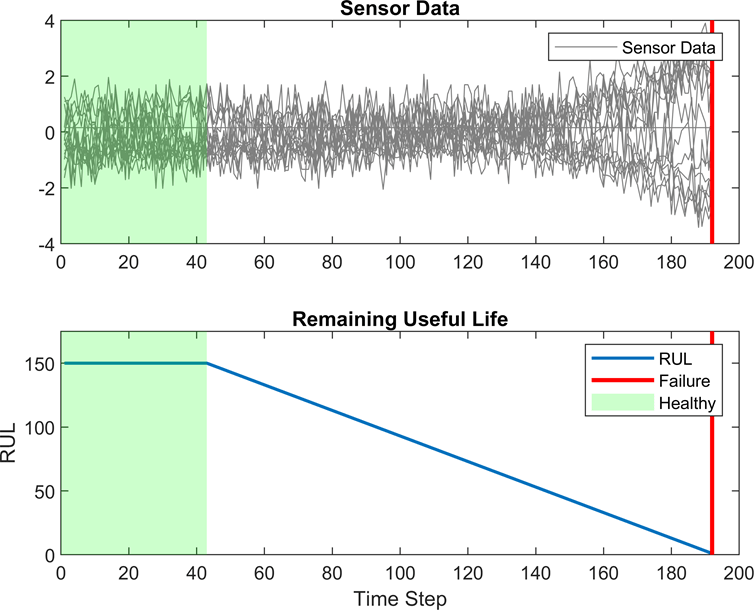
RUL captures how many operational cycles an engine can make before failure. To focus on the sequence data from when the engines are close to failing, preprocess the data by clipping the responses at a specified threshold. This preprocessing operation allows the network to focus on predictor data behaviors close to failing by treating instances with higher RUL values as equal. For example, this figure shows the first response observation and the corresponding clipped response with a threshold of 150.
When you train a deep learning network, how you preprocess data, the number of layers and hidden units, and the initial learning rate in the network can affect the training behavior and performance of the network. Choosing the depth of an LSTM network involves balancing speed and accuracy. For example, deeper networks can be more accurate but take longer to train and converge [2].
By default, when you run a built-in training experiment for regression, Experiment Manager computes the loss and root mean squared error (RMSE) for each trial in your experiment. This example compares the performance of the network in each trial by using a custom metric that is specific to the problem data set. For more information on using custom metric functions, see Evaluate Deep Learning Experiments by Using Metric Functions.
Open Experiment
First, open the example. Experiment Manager loads a project with a preconfigured experiment. To open the experiment, in the Experiment Browser, double-click SequenceRegressionExperiment.

Built-in training experiments consist of a description, a table of hyperparameters, a setup function, and a collection of metric functions to evaluate the results of the experiment. Experiments that use Bayesian optimization include additional options to limit the duration of the experiment. For more information, see Train Network Using trainnet and Display Custom Metrics.
The Description field contains a textual description of the experiment. For this example, the description is:
Sequence-to-sequence regression to predict the remaining useful life (RUL) of engines. This experiment compares network performance using Bayesian optimization when changing data thresholding level, LSTM layer depth, the number of hidden units, and the initial learn rate.
The Hyperparameters section specifies the strategy and hyperparameter options to use for the experiment. For each hyperparameter, you can specify these options:
- Range — Enter a two-element vector that gives the lower bound and upper bound of a real- or integer-valued hyperparameter, or a string array or cell array that lists the possible values of a categorical hyperparameter.
- Type — Select
realfor a real-valued hyperparameter,integerfor an integer-valued hyperparameter, orcategoricalfor a categorical hyperparameter. - Transform — Select
noneto use no transform orlogto use a logarithmic transform. When you selectlog, the hyperparameter values must be positive. With this setting, the Bayesian optimization algorithm models the hyperparameter on a logarithmic scale.
When you run the experiment, Experiment Manager searches for the best combination of hyperparameters. Each trial uses a new combination of the hyperparameter values based on the results of the previous trials. This example uses these hyperparameters:
Thresholdsets all response data above the threshold value to be equal to the threshold value. To prevent uniform response data, use threshold values greater than or equal to 150. To limit the set of allowable values to 150, 200 and 250, the experiment modelsThresholdas a categorical hyperparameter.LSTMDepthindicates the number of LSTM layers used in the network. Specify this hyperparameter as an integer between 1 and 3.NumHiddenUnitsdetermines the number of hidden units, or the amount of information stored at each time step, used in the network. Increasing the number of hidden units can result in overfitting the data and in a longer training time. Decreasing the number of hidden units can result in underfitting the data. Specify this hyperparameter as an integer between 50 and 300.InitialLearnRatespecifies the initial learning rate used for training. If the learning rate is too low, then training takes a long time. If the learning rate is too high, then training can reach a suboptimal result or diverge. The best learning rate depends on your data as well as the network you are training. The experiment models this hyperparameter on a logarithmic scale because the range of values (0.001 to 0.1) spans several orders of magnitude.
Under Bayesian Optimization Options, you can specify the duration of the experiment by entering the maximum time (in seconds) and the maximum number of trials to run. To best use the power of Bayesian optimization, perform at least 30 objective function evaluations.
The Setup Function section specifies a function that configures the training data, network architecture, and training options for the experiment. To open this function in MATLAB® Editor, click Edit. The code for the function also appears in Setup Function. The input to the setup function is a structure with fields from the hyperparameter table. The function returns four outputs that you use to train a network for image regression problems. In this example, the setup function has these sections:
- Load and Preprocess Data downloads and extracts the Turbofan Engine Degradation Simulation data set. This section of the setup function also filters out constant valued features, normalizes the predictor data to have zero mean and unit variance, clips the response data by using the numerical value of the hyperparameter
Threshold, and randomly selects training examples to use for validation.
filename = matlab.internal.examples.downloadSupportFile("nnet", ... "data/TurbofanEngineDegradationSimulationData.zip"); dataFolder = fullfile(tempdir,"turbofan"); if ~exist(dataFolder,"dir") unzip(filename,dataFolder); end
filenameTrainPredictors = fullfile(dataFolder,"train_FD001.txt"); [XTrain,YTrain] = processTurboFanDataTrain(filenameTrainPredictors);
XTrain = helperFilter(XTrain); XTrain = helperNormalize(XTrain);
thr = str2double(params.Threshold); for i = 1:numel(YTrain) YTrain{i}(YTrain{i} > thr) = thr; end
for i=1:numel(XTrain) sequence = XTrain{i}; sequenceLengths(i) = size(sequence,2); end
[~,idx] = sort(sequenceLengths,"descend"); XTrain = XTrain(idx); YTrain = YTrain(idx);
idx = randperm(numel(XTrain),10); XValidation = XTrain(idx); XTrain(idx) = []; YValidation = YTrain(idx); YTrain(idx) = [];
- Define Network Architecture defines the architecture for an LSTM network for sequence-to-sequence regression. The network consists of LSTM layers followed by a fully connected layer of size 100 and a dropout layer with a dropout probability of 0.5. The hyperparameters
LSTMDepthandNumHiddenUnitsspecify the number of LSTM layers and the number of hidden units for each layer.
numResponses = size(YTrain{1},1); featureDimension = size(XTrain{1},1); LSTMDepth = params.LSTMDepth; numHiddenUnits = params.NumHiddenUnits;
layers = sequenceInputLayer(featureDimension);
for i = 1:LSTMDepth layers = [layers;lstmLayer(numHiddenUnits,OutputMode="sequence")]; end
layers = [layers fullyConnectedLayer(100) reluLayer() dropoutLayer(0.5) fullyConnectedLayer(numResponses) regressionLayer];
- Specify Training Options defines the training options for the experiment. Because deeper networks take longer to converge, the number of epochs is set to 300 to ensure all network depths converge. This example validates the network every 30 iterations. The initial learning rate equals the
InitialLearnRatevalue from the hyperparameter table and drops by a factor of 0.2 every 15 epochs. With the training optionExecutionEnvironmentset to"auto", the experiment runs on a GPU if one is available. Otherwise, Experiment Manager uses the CPU. Because this example compares network depths and trains for many epochs, using a GPU speeds up training time considerably. Using a GPU requires Parallel Computing Toolbox™ and a supported GPU device. For more information, see GPU Computing Requirements (Parallel Computing Toolbox).
maxEpochs = 300; miniBatchSize = 20;
options = trainingOptions("adam", ... ExecutionEnvironment="auto", ... MaxEpochs=maxEpochs, ... MiniBatchSize=miniBatchSize, ... ValidationData={XValidation,YValidation}, ... ValidationFrequency=30, ... InitialLearnRate=params.InitialLearnRate, ... LearnRateDropFactor=0.2, ... LearnRateDropPeriod=15, ... GradientThreshold=1, ... Shuffle="never", ... Verbose=false);
The Metrics section specifies optional functions that evaluate the results of the experiment. Experiment Manager evaluates these functions each time it finishes training the network. This example includes a metric function MeanMaxAbsoluteError that identifies networks that underpredict or overpredict the RUL. If the prediction underestimates the RUL, engine maintenance might be scheduled before it is necessary. If the prediction overestimates the RUL, the engine might fail while in operation, resulting in high costs or safety concerns. To help mitigate these scenarios, the MeanMaxAbsoluteError metric calculates the maximum absolute error, averaged across the entire training set. This metric calls the [predict](../ref/seriesnetwork.predict.html) function to make a sequence of RUL predictions from the training set. Then, after calculating the maximum absolute error between each training response and predicted response sequence, the metric function computes the mean of all maximum absolute errors and identifies the maximum deviations between the actual and predicted responses. To open this function in MATLAB Editor, select the name of the metric function and click Edit. The code for the function also appears in Compute Mean of Maximum Absolute Errors.
Run Experiment
When you run the experiment, Experiment Manager searches for the best combination of hyperparameters with respect to the chosen metric. Each trial in the experiment uses a new combination of hyperparameter values based on the results of the previous trials.
Training can take some time. To limit the duration of the experiment, you can modify the Bayesian Optimization Options by reducing the maximum running time or the maximum number of trials. However, note that running fewer than 30 trials can prevent the Bayesian optimization algorithm from converging to an optimal set of hyperparameters.
By default, Experiment Manager runs one trial at a time. If you have Parallel Computing Toolbox™, you can run multiple trials at the same time or offload your experiment as a batch job in a cluster:
- To run one trial of the experiment at a time, on the Experiment Manager toolstrip, set Mode to
Sequentialand click Run. - To run multiple trials at the same time, set Mode to
Simultaneousand click Run. If there is no current parallel pool, Experiment Manager starts one using the default cluster profile. Experiment Manager then runs as many simultaneous trials as there are workers in your parallel pool. For best results, before you run your experiment, start a parallel pool with as many workers as GPUs. For more information, see Run Experiments in Parallel and GPU Computing Requirements (Parallel Computing Toolbox). - To offload the experiment as a batch job, set Mode to
Batch SequentialorBatch Simultaneous, specify your cluster and pool size, and click Run. For more information, see Offload Experiments as Batch Jobs to a Cluster.
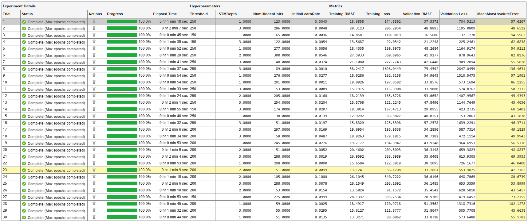
A table of results displays the metric function values for each trial. Experiment Manager highlights the trial with the optimal value for the selected metric. For example, in this experiment, the 23rd trial produces the smallest maximum absolute error.
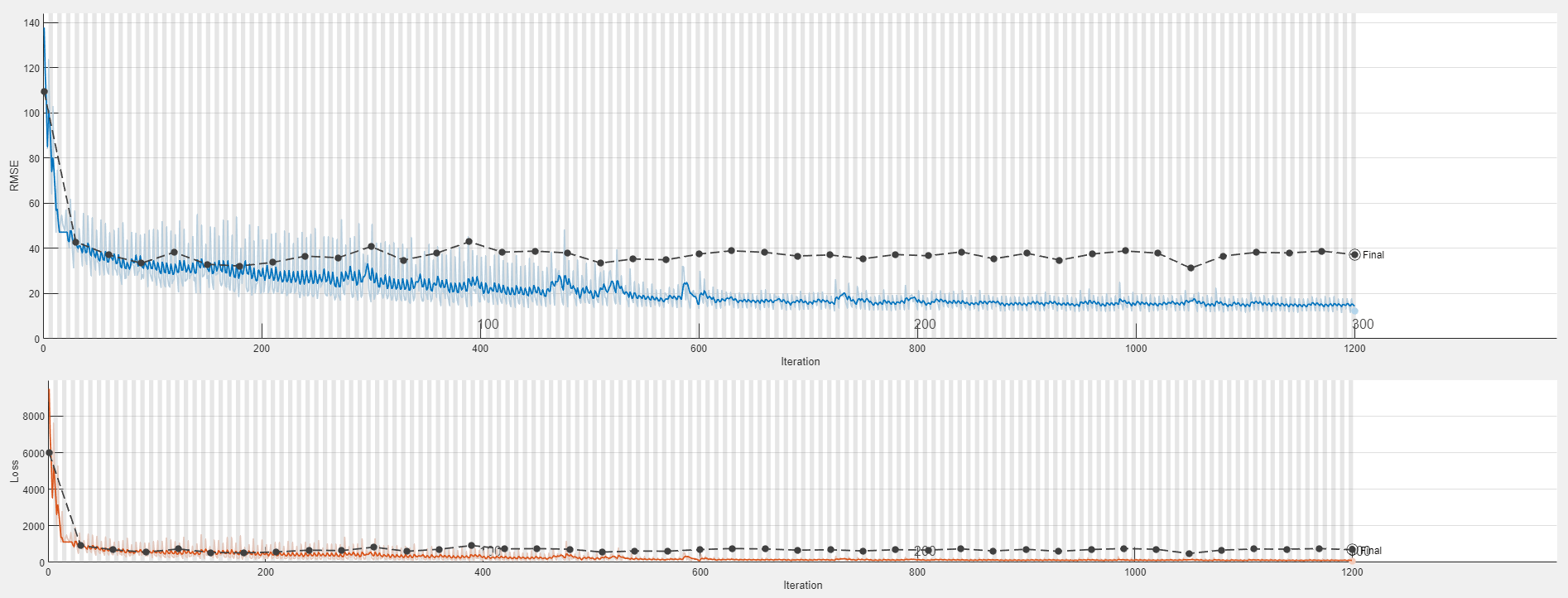
To display the training plot and track the progress of each trial while the experiment is running, under Review Results, click Training Plot. The elapsed time for a trial to complete training increases with network depth.
Evaluate Results
In the table of results, the MeanMaxAbsoluteError value quantifies how much the network underpredicts or overpredicts the RUL. The Validation RMSE value quantifies how well the network generalizes to unseen data. To find the best result for your experiment, sort the table of results and select the trial that has the lowest MeanMaxAbsoluteError and Validation RMSE values:
- Point to the MeanMaxAbsoluteError column.
- Click the triangle icon.
- Select Sort in Ascending Order.
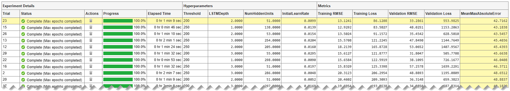
Similarly, find the trial with the smallest validation RMSE by opening the drop-down menu for the Validation RMSE column and selecting Sort in Ascending Order.
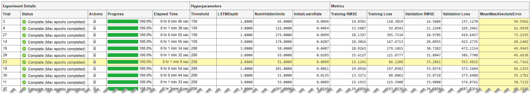
If no single trial minimizes both values, opt for a trial that ranks well for both metrics. For instance, in these results, trial 23 has the smallest mean maximum absolute error and the seventh smallest validation RMSE. Among the trials with a lower validation RMSE, only trial 29 has a comparable mean maximum absolute error. Which of these trials is preferable depends on whether you favor a lower mean maximum absolute error or a lower validation RMSE.
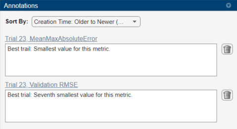
To record observations about the results of your experiment, add an annotation:
- In the results table, right-click the MeanMaxAbsoluteError cell of the best trial.
- Select Add Annotation.
- In the Annotations pane, enter your observations in the text box.
- Repeat the previous steps for the Validation RMSE cell.
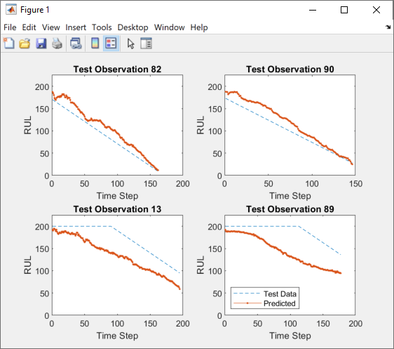
To test the best trial in your experiment, export the trained networks and display the predicted response sequence for several randomly chosen test sequences:
- Select the best trial in your experiment.
- On the Experiment Manager toolstrip, click Export > Trained Network.
- In the dialog window, enter the name of a workspace variable for the exported network. The default name is
trainedNetwork. - In the MATLAB Command Window, use the exported network and the
Thresholdvalue of the network as inputs to the helper functionplotSequences:
plotSequences(trainedNetwork,200)
To view the code for this function, see Plot Predictive Maintenance Sequences. The function plots the true and predicted response sequences of unseen test data.
Close Experiment
In the Experiment Browser, right-click TurbofanSequenceRegressionProject and select Close Project. Experiment Manager closes the experiment and results contained in the project.
Setup Function
This function configures the training data, network architecture, and training options for the experiment. The input to this function is a structure with fields from the hyperparameter table. The function returns four outputs that you use to train a network for image regression problems.
function [XTrain,YTrain,layers,options] = SequenceRegressionExperiment_setup(params)
Load and Preprocess Data
filename = matlab.internal.examples.downloadSupportFile("nnet", ... "data/TurbofanEngineDegradationSimulationData.zip"); dataFolder = fullfile(tempdir,"turbofan"); if ~exist(dataFolder,"dir") unzip(filename,dataFolder); end
filenameTrainPredictors = fullfile(dataFolder,"train_FD001.txt"); [XTrain,YTrain] = processTurboFanDataTrain(filenameTrainPredictors);
XTrain = helperFilter(XTrain); XTrain = helperNormalize(XTrain);
thr = str2double(params.Threshold); for i = 1:numel(YTrain) YTrain{i}(YTrain{i} > thr) = thr; end
for i=1:numel(XTrain) sequence = XTrain{i}; sequenceLengths(i) = size(sequence,2); end
[~,idx] = sort(sequenceLengths,"descend"); XTrain = XTrain(idx); YTrain = YTrain(idx);
idx = randperm(numel(XTrain),10); XValidation = XTrain(idx); XTrain(idx) = []; YValidation = YTrain(idx); YTrain(idx) = [];
Define Network Architecture
numResponses = size(YTrain{1},1); featureDimension = size(XTrain{1},1); LSTMDepth = params.LSTMDepth; numHiddenUnits = params.NumHiddenUnits;
layers = sequenceInputLayer(featureDimension);
for i = 1:LSTMDepth layers = [layers;lstmLayer(numHiddenUnits,OutputMode="sequence")]; end
layers = [layers fullyConnectedLayer(100) reluLayer() dropoutLayer(0.5) fullyConnectedLayer(numResponses) regressionLayer];
Specify Training Options
maxEpochs = 300; miniBatchSize = 20;
options = trainingOptions("adam", ... ExecutionEnvironment="auto", ... MaxEpochs=maxEpochs, ... MiniBatchSize=miniBatchSize, ... ValidationData={XValidation,YValidation}, ... ValidationFrequency=30, ... InitialLearnRate=params.InitialLearnRate, ... LearnRateDropFactor=0.2, ... LearnRateDropPeriod=15, ... GradientThreshold=1, ... Shuffle="never", ... Verbose=false);
Filter and Normalize Predictive Maintenance Data
The helper function helperFilter filters the data by removing features with constant values. Features that remain constant for all time steps can negatively impact the training.
function [XTrain,XTest] = helperFilter(XTrain,XTest)
m = min([XTrain{:}],[],2); M = max([XTrain{:}],[],2); idxConstant = M == m;
for i = 1:numel(XTrain) XTrain{i}(idxConstant,:) = []; if nargin>1 XTest{i}(idxConstant,:) = []; end end end
The helper function helperNormalize normalizes the training and test predictors to have zero mean and unit variance.
function [XTrain,XTest] = helperNormalize(XTrain,XTest)
mu = mean([XTrain{:}],2); sig = std([XTrain{:}],0,2);
for i = 1:numel(XTrain) XTrain{i} = (XTrain{i} - mu) ./ sig; if nargin>1 XTest{i} = (XTest{i} - mu) ./ sig; end end end
Compute Mean of Maximum Absolute Errors
This metric function calculates the maximum absolute error of the trained network, averaged over the training set.
function metricOutput = MeanMaxAbsoluteError(trialInfo)
net = trialInfo.trainedNetwork; thr = str2double(trialInfo.parameters.Threshold);
filenamePredictors = fullfile(tempdir,"turbofan","train_FD001.txt"); [XTrain,YTrain] = processTurboFanDataTrain(filenamePredictors); XTrain = helperFilter(XTrain); XTrain = helperNormalize(XTrain);
for i = 1:numel(YTrain) YTrain{i}(YTrain{i} > thr) = thr; end
YPred = predict(net,XTrain,MiniBatchSize=1);
maxAbsErrors = zeros(1,numel(YTrain)); for i=1:numel(YTrain) absError = abs(YTrain{i}-YPred{i}); maxAbsErrors(i) = max(absError); end
metricOutput = mean(maxAbsErrors); end
Plot Predictive Maintenance Sequences
This function plots the true and predicted response sequences to allow you to evaluate the performance of your trained network. This function uses the helper functions helperFilter and helperNormalize. To view the code for these functions, see Filter and Normalize Predictive Maintenance Data.
function plotSequences(net,threshold)
filenameTrainPredictors = fullfile(tempdir,"turbofan","train_FD001.txt"); filenameTestPredictors = fullfile(tempdir,"turbofan","test_FD001.txt"); filenameTestResponses = fullfile(tempdir,"turbofan","RUL_FD001.txt");
[XTrain,YTrain] = processTurboFanDataTrain(filenameTrainPredictors); [XTest,YTest] = processTurboFanDataTest(filenameTestPredictors,filenameTestResponses); [XTrain,XTest] = helperFilter(XTrain,XTest); [~,XTest] = helperNormalize(XTrain,XTest);
for i = 1:numel(YTrain) YTrain{i}(YTrain{i} > threshold) = threshold; YTest{i}(YTest{i} > threshold) = threshold; end
YPred = predict(net,XTest,MiniBatchSize=1);
idx = randperm(100,4); figure for i = 1:numel(idx) subplot(2,2,i) plot(YTest{idx(i)},"--") hold on plot(YPred{idx(i)},".-") hold off ylim([0 threshold+25]) title("Test Observation " + idx(i)) xlabel("Time Step") ylabel("RUL") end legend(["Test Data" "Predicted"],Location="southwest") end
References
[1] Saxena, Abhinav, Kai Goebel, Don Simon, and Neil Eklund. "Damage Propagation Modeling for Aircraft Engine Run-to-Failure Simulation." 2008 International Conference on Prognostics and Health Management (2008): 1–9.
[2] Jozefowicz, Rafal, Wojciech Zaremba, and Ilya Sutskever. "An Empirical Exploration of Recurrent Network Architectures."Proceedings of the 32nd International Conference on Machine Learning (2015): 2342–2350.
See Also
Apps
Functions
Related Topics
- Long Short-Term Memory Neural Networks
- Sequence-to-Sequence Regression Using Deep Learning
- Sequence-to-One Regression Using Deep Learning
- Tune Experiment Hyperparameters by Using Bayesian Optimization
- Evaluate Deep Learning Experiments by Using Metric Functions
- Run Experiments in Parallel
- Offload Experiments as Batch Jobs to a Cluster