Test Generated Code with SIL and PIL Simulations - MATLAB & Simulink (original) (raw)
Test numerical equivalence between model components and production code that you generate from the components by using software-in-the-loop (SIL) and processor-in-the-loop (PIL) simulations.
With a SIL simulation, you test source code on your development computer. With a PIL simulation, you test the compiled object code that you intend to deploy in production by running the object code on real target hardware or an instruction set simulator. To determine whether model components and generated code are numerically equivalent, compare SIL and PIL results against normal mode results.
This example shows three ways of running SIL and PIL simulations. You can use the top model, Model blocks, or SIL and PIL blocks that you create from a subsystem. See Choose a SIL or PIL Approach.
Target Connectivity Configuration for PIL
Before you can run PIL simulations, you must configure target connectivity. The target connectivity configuration enables the PIL simulation to:
- Build the target application.
- Download, start, and stop the application on the target.
- Support communication between Simulink and the target.
To produce a target connectivity configuration, you can use the supplied target connectivity API. For details, see Create PIL Target Connectivity Configuration for Simulink.
For supported hardware, you can use target support packages. For details, see Embedded Coder Supported Hardware.
SIL or PIL Simulation with a Top Model
Test generated model code by running a top-model SIL or PIL simulation. With this approach:
- You test code generated from the top model, which uses the standalone code interface.
- You configure the model to load test vectors or stimulus inputs from the MATLAB workspace.
- You can easily switch the top model between the normal, SIL, and PIL simulation modes.
Open a simple counter top model.
model='SILTopModel'; close_system(model,0) open_system(model)
To focus on numerical equivalence testing, turn off:
- Model coverage
- Code coverage
- Execution time profiling
set_param(gcs, 'RecordCoverage','off'); coverageSettings = get_param(model, 'CodeCoverageSettings'); coverageSettings.CoverageTool='None'; set_param(model, 'CodeCoverageSettings',coverageSettings); set_param(model, 'CodeExecutionProfiling','off');
Configure the input stimulus data.
[ticks_to_count, reset, counter_mode, count_enable] = ... SILTopModelData(T);
Configure logging options in the model.
set_param(model, 'LoadExternalInput','on'); set_param(model, 'ExternalInput','ticks_to_count, reset, counter_mode, count_enable'); set_param(model, 'SignalLogging', 'on'); set_param(model, 'SignalLoggingName', 'logsOut'); set_param(model, 'SaveOutput','on')
Run a normal mode simulation.
set_param(model,'SimulationMode','normal') sim_output = sim(model,10); yout_normal = [sim_output.yout.signals(1).values sim_output.yout.signals(2).values];
Run a top-model SIL simulation.
set_param(model,'SimulationMode','Software-in-the-Loop (SIL)') sim_output = sim(model,10);
Searching for referenced models in model 'SILTopModel'.
Total of 1 models to build.
Starting build procedure for: SILTopModel
Successful completion of build procedure for: SILTopModel
Build Summary
Top model targets:
Model Build Reason Status Build Duration
SILTopModel Information cache folder or artifacts were missing. Code generated and compiled. 0h 0m 9.6222s
1 of 1 models built (0 models already up to date) Build duration: 0h 0m 10.095s
Preparing to start SIL simulation ...
Building with 'gcc'. MEX completed successfully.
Updating code generation report with SIL files ...
Starting SIL simulation for component: SILTopModel
Application stopped
Stopping SIL simulation for component: SILTopModel
yout_sil = [sim_output.yout.signals(1).values sim_output.yout.signals(2).values];
Unless up-to-date code for this model exists, new code is generated and compiled. The generated code runs as a separate process on your computer.
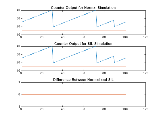
Plot and compare the results of the normal and SIL simulations. Observe that the results match.
fig1 = figure; subplot(3,1,1), plot(yout_normal), title('Counter Output for Normal Simulation') subplot(3,1,2), plot(yout_sil), title('Counter Output for SIL Simulation') subplot(3,1,3), plot(yout_normal-yout_sil), ... title('Difference Between Normal and SIL');
Clean up.
close_system(model,0); if ishandle(fig1), close(fig1), end clear fig1 simResults = {'yout_sil','yout_normal','model','T',... 'ticks_to_count','reset'}; save([model '_results'],simResults{:}); clear(simResults{:},'simResults')
SIL or PIL Simulation with a Model Block
Test generated model code by using a test harness model that runs a Model block in SIL mode. With this approach:
- You can test code that is generated from a top model or a referenced model. The code from the top model uses the standalone code interface. The code from the referenced model uses the model reference code interface. For more information, see Code Interfaces for SIL and PIL.
- You use a test harness model or a system model to provide test vector or stimulus inputs.
- You can easily switch a Model block between the normal, SIL, and PIL simulation modes.
Open an example model that has two Model blocks which reference the same model. In a simulation, you run one Model block in SIL mode and the other Model block in normal mode.
model='SILModelBlock'; open_system(model);
Turn off:
- Code coverage
- Execution time profiling
coverageSettings = get_param(model, 'CodeCoverageSettings'); coverageSettings.CoverageTool='None'; set_param(model, 'CodeCoverageSettings',coverageSettings); open_system('SILModelBlock') set_param('SILModelBlock', 'CodeExecutionProfiling','off'); open_system('SILCounter') set_param('SILCounter', 'CodeExecutionProfiling','off'); currentFolder=pwd; save_system('SILCounter', fullfile(currentFolder,'SILCounter.slx'))
Configure state logging for the models.
set_param('SILCounter', 'SaveFormat','Dataset'); save_system('SILCounter', fullfile(currentFolder,'SILCounter.slx')) set_param(model, 'SaveFormat','Dataset'); set_param(model, 'SaveState','on'); set_param(model, 'StateSaveName', 'xout');
Test Top-Model Code
For the Model block in SIL mode, specify generation of top-model code, which uses the standalone code interface.
set_param([model '/CounterA'], 'CodeInterface', 'Top model');
Run a simulation of the test harness model.
Searching for referenced models in model 'SILModelBlock'.
Total of 1 models to build.
Searching for referenced models in model 'SILCounter'.
Total of 1 models to build.
Starting build procedure for: SILCounter
Successful completion of build procedure for: SILCounter
Build Summary
Top model targets:
Model Build Reason Status Build Duration
SILCounter Information cache folder or artifacts were missing. Code generated and compiled. 0h 0m 8.061s
1 of 1 models built (0 models already up to date) Build duration: 0h 0m 8.5171s
Preparing to start SIL simulation ...
Building with 'gcc'. MEX completed successfully.
Updating code generation report with SIL files ...
Starting SIL simulation for component: SILCounter
Application stopped
Stopping SIL simulation for component: SILCounter
The model block in SIL mode runs as a separate process on your computer. In the working folder, you see that standalone code is generated for the referenced model unless generated code from a previous build exists.
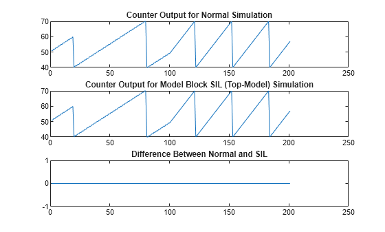
Compare the behavior of Model blocks in normal and SIL modes. The results match.
yout = out.logsOut; yout_sil = yout.get('counterA').Values.Data; yout_normal = yout.get('counterB').Values.Data; fig1 = figure; subplot(3,1,1), plot(yout_normal), title('Counter Output for Normal Simulation') subplot(3,1,2), ... plot(yout_sil), title('Counter Output for Model Block SIL (Top-Model) Simulation') subplot(3,1,3), plot(yout_normal-yout_sil), ... title('Difference Between Normal and SIL');
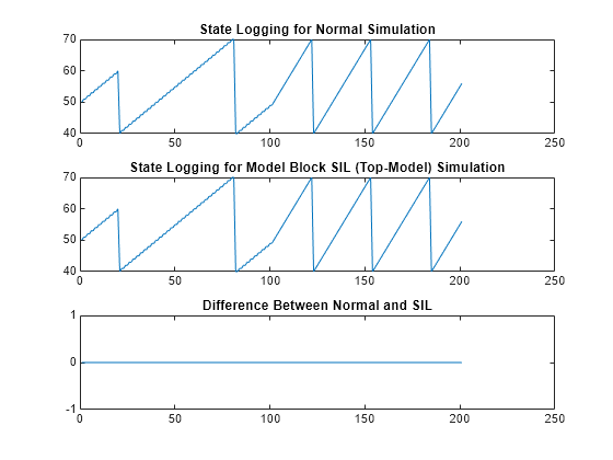
Compare the logged states of Model blocks from normal and SIL mode simulations.
xout = out.xout; xout_sil = xout{1}.Values.Data; xout_normal = xout{2}.Values.Data; fig1 = figure; subplot(3,1,1), plot(xout_sil), title('State Logging for Normal Simulation') subplot(3,1,2), ... plot(xout_normal), title('State Logging for Model Block SIL (Top-Model) Simulation') subplot(3,1,3), plot(xout_normal-xout_sil), ... title('Difference Between Normal and SIL');
Test Model Reference Code
For the Model block in SIL mode, specify generation of referenced model code, which uses the model reference code interface.
set_param([model '/CounterA'], 'CodeInterface', 'Model reference');
Run a simulation of the test harness model.
Searching for referenced models in model 'SILModelBlock'.
Total of 1 models to build.
Starting serial code generation build.
Starting build procedure for: SILCounter
Successful completion of build procedure for: SILCounter
Build Summary
Model reference code generation targets:
Model Build Reason Status Build Duration
SILCounter Target (SILCounter.c) did not exist. Code generated and compiled. 0h 0m 6.2851s
1 of 1 models built (0 models already up to date) Build duration: 0h 0m 6.7869s
Preparing to start SIL simulation ...
Building with 'gcc'. MEX completed successfully.
Updating code generation report with SIL files ...
Starting SIL simulation for component: SILCounter
Application stopped
Stopping SIL simulation for component: SILCounter
The model block in SIL mode runs as a separate process on your computer. In the working folder, you see that model reference code is generated unless code from a previous build exists.
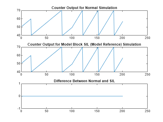
Compare the behavior of Model blocks in normal and SIL modes. The results match.
yout2 = out2.logsOut; yout2_sil = yout2.get('counterA').Values.Data; yout2_normal = yout2.get('counterB').Values.Data; fig1 = figure; subplot(3,1,1), plot(yout2_normal), title('Counter Output for Normal Simulation') subplot(3,1,2), ... plot(yout2_sil), title('Counter Output for Model Block SIL (Model Reference) Simulation') subplot(3,1,3), plot(yout2_normal-yout2_sil), ... title('Difference Between Normal and SIL');
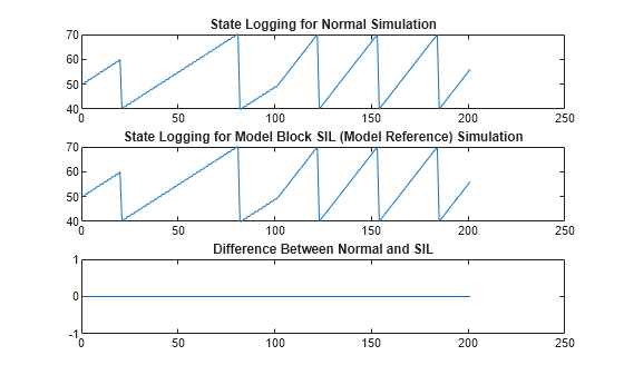
Compare the logged states of Model blocks from normal and SIL mode simulations.
xout2 = out.xout; xout2_sil = xout2{1}.Values.Data; xout2_normal = xout2{2}.Values.Data; fig1 = figure; subplot(3,1,1), plot(xout2_sil), title('State Logging for Normal Simulation') subplot(3,1,2), ... plot(xout2_normal), title('State Logging for Model Block SIL (Model Reference) Simulation') subplot(3,1,3), plot(xout2_normal-xout2_sil), ... title('Difference Between Normal and SIL');
Clean up.
close_system(model,0); if ishandle(fig1), close(fig1), end, clear fig1 simResults={'out','yout','yout_sil','yout_normal', ... 'out2','yout2','yout2_sil','yout2_normal', ... 'SilCounterBus','T','reset','ticks_to_count','Increment'}; save([model '_results'],simResults{:}); clear(simResults{:},'simResults')
SIL or PIL Block Simulation
Test generated subsystem code by using a SIL or PIL block in a simulation. With this approach:
- You test code generated from subsystems, which uses the standalone code interface.
- You provide a test harness or a system model to supply test vector or stimulus inputs.
- You replace your original subsystem with the generated SIL or PIL block.
Open a simple model, which consists of a control algorithm and a plant model in a closed loop. The control algorithm regulates the output from the plant.
model='SILBlock'; close_system(model,0) open_system(model)
Run a normal mode simulation
out = sim(model,10); yout_normal = out.yout; clear out
Configure the build process to create the SIL block for testing.
set_param(model,'CreateSILPILBlock','SIL');
To test the behavior on production hardware, specify a PIL block.
To create the SIL block, generate code for the control algorithm subsystem. You see the SIL block at the end of the build process. Its input and output ports match those of the control algorithm subsystem.
close_system('untitled',0); slbuild([model '/Controller'])
Searching for referenced models in model 'Controller'.
Total of 1 models to build.
Starting build procedure for: Controller
Successful completion of build procedure for: Controller
Creating SIL block ...
Building with 'gcc'. MEX completed successfully.
Build Summary
Top model targets:
Model Build Reason Status Build Duration
Controller Information cache folder or artifacts were missing. Code generated and compiled. 0h 0m 7.6175s
1 of 1 models built (0 models already up to date) Build duration: 0h 0m 15.187s
Alternatively, you can right-click the subsystem and select C/C++ Code > Build This Subsystem. In the dialog box that opens, click Build.
To perform a SIL simulation of the controller and plant model in a closed loop, replace the original control algorithm with the new SIL block. To avoid losing your original subsystem, do not save your model in this state.
controllerBlock = [model '/Controller']; blockPosition = get_param(controllerBlock,'Position'); delete_block(controllerBlock); add_block('untitled/Controller',[controllerBlock '(SIL)'],... 'Position', blockPosition); close_system('untitled',0); clear controllerBlock blockPosition
Run the SIL simulation.
Preparing to start SIL block simulation: SILBlock/Controller(SIL) ...
Starting SIL simulation for component: SILBlock
Application stopped
Stopping SIL simulation for component: SILBlock
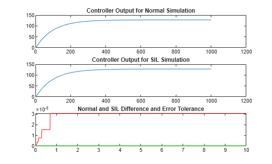
The control algorithm uses single-precision, floating-point arithmetic. You can expect the order of magnitude for differences between SIL and normal simulations to be close to the machine precision for single-precision data.
Define an error tolerance for SIL simulation results that is based on the machine precision for the single-precision, normal simulation results.
machine_precision = eps(single(yout_normal)); tolerance = 4 * machine_precision;
Compare normal and SIL simulation results. In the third plot, the differences between the simulations lie well within the defined error tolerance.
yout_sil = out.yout; tout = out.tout; fig1 = figure; subplot(3,1,1), plot(yout_normal), title('Controller Output for Normal Simulation') subplot(3,1,2), plot(yout_sil), title('Controller Output for SIL Simulation') subplot(3,1,3), plot(tout,abs(yout_normal-yout_sil),'g-', tout,tolerance,'r-'), ... title('Normal and SIL Difference and Error Tolerance');
Clean up.
close_system(model,0); if ishandle(fig1), close(fig1), end clear fig1 simResults={'out','yout_sil','yout_normal','tout','machine_precision'}; save([model '_results'],simResults{:}); clear(simResults{:},'simResults')
Hardware Implementation Settings
When you run a SIL simulation, you must configure your hardware implementation settings (characteristics such as native word sizes) to allow compilation for your development computer. These settings can differ from the hardware implementation settings that you use when building the model for your production hardware. To avoid the need to change hardware implementation settings between SIL and PIL simulations, enable portable word sizes. For more information, see Configure Hardware Implementation Settings.