matlab.perftest.TestCase - Class for writing tests with performance testing framework - MATLAB (original) (raw)
Namespace: matlab.perftest
Superclasses: matlab.unittest.TestCase
Class for writing tests with performance testing framework
Description
The matlab.perftest.TestCase class lets you write class-based performance tests and define boundaries that restrict measurements to specific code segments. Because thematlab.perftest.TestCase class derives from thematlab.unittest.TestCase class, your tests have access to the features of the unit testing framework. Therefore, you can perform qualifications within your performance tests to ensure correct functional behavior while measuring code performance. For more information about creating and running performance tests, see Overview of Performance Testing Framework.
The performance testing framework automatically createsmatlab.perftest.TestCase instances when running the tests.
The matlab.perftest.TestCase class is a handle class.
Examples
Compare the performance of various preallocation approaches by creating a test class that derives from matlab.perftest.TestCase.
In a file named preallocationTest.m in your current folder, create the preallocationTest test class. The class contains four Test methods that correspond to different approaches to creating a vector of ones. When you run any of these methods with the runperf function, the function measures the time it takes to run the code inside the method.
classdef preallocationTest < matlab.perftest.TestCase methods (Test) function testOnes(testCase) x = ones(1,1e7); end
    function testIndexingWithVariable(testCase)
        id = 1:1e7;
        x(id) = 1;
    end

    function testIndexingOnLHS(testCase)
        x(1:1e7) = 1;
    end

    function testForLoop(testCase)
        for i = 1:1e7
            x(i) = 1;
        end
    end
end
end
Run performance tests for all the tests with "Indexing" in their name. Your results might vary, and you might see a warning if runperf does not meet statistical objectives.
results = runperf("preallocationTest","Name","Indexing")
Running preallocationTest .......... .......... .......... .. Done preallocationTest
results = 1×2 TimeResult array with properties:
Name
Valid
Samples
TestActivity
Totals: 2 Valid, 0 Invalid. 3.011 seconds testing time.
To compare the preallocation methods, create a table of summary statistics from results. In this example, the testIndexingOnLHS method was the faster way to initialize the vector to ones.
T = sampleSummary(results)
T=2×7 table
Name SampleSize Mean StandardDeviation Min Median Max
__________________________________________ __________ ________ _________________ ________ ________ ________
preallocationTest/testIndexingWithVariable        17          0.1223         0.014378         0.10003     0.12055     0.15075
preallocationTest/testIndexingOnLHS                5        0.027557        0.0013247        0.026187    0.027489    0.029403
Visualize the computational complexity of two sorting algorithms, bubble sort and merge sort, which sort list elements in ascending order. Bubble sort is a simple sorting algorithm that repeatedly steps through a list, compares adjacent pairs of elements, and swaps elements if they are in the wrong order. Merge sort is a "divide and conquer" algorithm that takes advantage of the ease of merging sorted sublists into a new sorted list.
In a file named bubbleSort.m in your current folder, create thebubbleSort function, which implements the bubble sort algorithm.
function y = bubbleSort(x) % Sorting algorithm with O(n^2) complexity n = length(x); swapped = true;
while swapped swapped = false; for i = 2:n if x(i-1) > x(i) temp = x(i-1); x(i-1) = x(i); x(i) = temp; swapped = true; end end end
y = x; end
In a file named mergeSort.m in your current folder, create themergeSort function, which implements the merge sort algorithm.
function y = mergeSort(x) % Sorting algorithm with O(n*logn) complexity y = x; % A list of one element is considered sorted
if length(x) > 1 mid = floor(length(x)/2); L = x(1:mid); R = x((mid+1):end);
% Sort left and right sublists recursively
L = mergeSort(L);
R = mergeSort(R);

% Merge the sorted left (L) and right (R) sublists
i = 1;
j = 1;
k = 1;
while i <= length(L) && j <= length(R)
    if L(i) < R(j)
        y(k) = L(i);
        i = i + 1;
    else
        y(k) = R(j);
        j = j + 1;
    end
    k = k + 1;
end

% At this point, either L or R is empty
while i <= length(L)
    y(k) = L(i);
    i = i + 1;
    k = k + 1;
end

while j <= length(R)
    y(k) = R(j);
    j = j + 1;
    k = k + 1;
end
end
end
In a file named SortTest.m in your current folder, create theSortTest parameterized test class, which compares the performance of the bubble sort and merge sort algorithms. The len property of the class contains the numbers of list elements you want to test with.
classdef SortTest < matlab.perftest.TestCase properties Data SortedData end
properties (ClassSetupParameter)
    % Create 25 logarithmically spaced values between 10^2 and 10^4
    len = num2cell(round(logspace(2,4,25)));
end

methods (TestClassSetup)
    function ClassSetup(testCase,len)
        orig = rng;
        testCase.addTeardown(@rng,orig)
        rng("default")
        testCase.Data = rand(1,len);
        testCase.SortedData = sort(testCase.Data);
    end
end

methods (Test)
    function testBubbleSort(testCase)
        while testCase.keepMeasuring
            y = bubbleSort(testCase.Data);
        end
        testCase.verifyEqual(y,testCase.SortedData)
    end

    function testMergeSort(testCase)
        while testCase.keepMeasuring
            y = mergeSort(testCase.Data);
        end
        testCase.verifyEqual(y,testCase.SortedData)
    end
end
end
Run performance tests for all the tests that correspond to thetestBubbleSort method and save the results in thebaseline array. Your results might vary from the results shown.
baseline = runperf("SortTest","ProcedureName","testBubbleSort");
Running SortTest .......... .......... .......... .......... .......... .......... .......... .......... .......... .......... .......... .......... .......... .......... .......... .......... .......... .......... .......... .......... .......... .......... .......... .......... .......... .......... .......... .......... .......... .. Done SortTest
Run performance tests for all the tests that correspond to thetestMergeSort method and save the results in themeasurement array.
measurement = runperf("SortTest","ProcedureName","testMergeSort");
Running SortTest .......... .......... .......... .......... .......... .......... .......... .......... .......... .......... .......... .......... .......... .......... .......... .......... .......... .......... .......... .......... .......... .......... .......... .......... .......... .......... .......... .......... .......... .......... .......... .......... .......... .......... .......... .......... .......... .......... .......... .......... .......... .......... .......... .......... .......... .......... .......... .......... .......... .......... .......... .......... .......... .......... .......... .......... .......... .......... .......... .......... .......... .......... .......... .......... .......... .......... .......... .......... .......... .......... .......... .......... .......... .......... .......... .......... .......... .......... .......... .......... .......... ..... Done SortTest
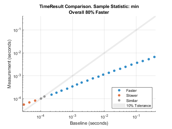
Visually compare the minimum of the MeasuredTime column in theSamples table for each corresponding pair ofbaseline and measurement objects. In this comparison plot, most data points are blue because they are below the shaded similarity region. This result indicates the superior performance of merge sort for the majority of tests. However, for small enough lists, bubble sort performs better than or comparable to merge sort, as shown by the orange and gray points in the plot. As a comparison summary, the plot reports that merge sort is 80% faster than bubble sort. This value is the geometric mean of the improvement percentages corresponding to all data points.
cp = comparisonPlot(baseline,measurement);
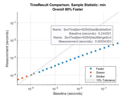
You can click or point to any data point to view detailed information about the time measurement results being compared.
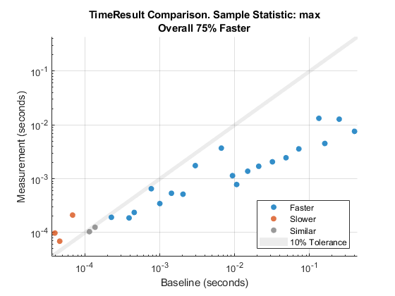
To study the worst-case sorting algorithm performance for different list lengths, create a comparison plot based on the maximum of sample measurement times.
cp = comparisonPlot(baseline,measurement,"max");
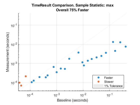
Reduce similarity tolerance to 0.01 when comparing the maximum of sample measurement times.
cp = comparisonPlot(baseline,measurement,"max","SimilarityTolerance",0.01);
Version History
Introduced in R2016a