Common Scope Block Tasks - MATLAB & Simulink (original) (raw)

To visualize your simulation results over time, use a Scope block or Time Scope (DSP System Toolbox) block

Connect Multiple Signals to Scope

To connect multiple signals to a scope, drag additional signals to the scope block. An additional port is created automatically.

To specify the number of input ports:

1. Open a scope window.
2. From the toolbar, select > .
3. Under General, in the Number of inputs box, enter the number of input ports, up to 96.

Signals from Nonvirtual Buses and Arrays of Buses

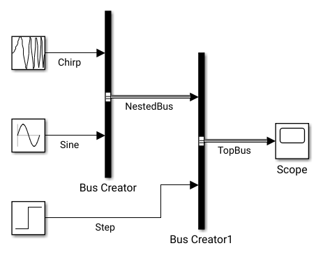
You can connect signals from nonvirtual buses and arrays of buses to aScope block. To display the bus signals, use normal or accelerator simulation mode. The Scope block displays each bus element in the order the elements appear in the bus, from the top to the bottom. Nested bus elements are flattened. For example, in this model, a Scope block is connected to a bus named TopBus, which contains the elementsNestedBus and Step.NestedBus connects to the first port of the Bus Creator block used to create TopBus, whileStep connects to the second port.NestedBus contains the Chirp andSine signals, with Chirp connected to the port above Sine in the Bus Creator block used to form NestedBus. In the Scope block, the two signals in NestedBus appear above the Step signal in the legend.

Save Simulation Data Using Scope Block

This example shows how to save signals to the MATLAB Workspace using the Scope block. You can us these steps for the Scope or Time Scope blocks. To save data from the Floating Scope or Scope viewer, see Save Simulation Data from Floating Scope.

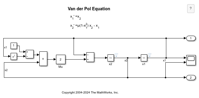
The vdp model represents the second-order Van der Pol (VDP) differential equation. For more information about the model, see Van der Pol Oscillator.

Log data to the workspace using the Scope block:

• Select Scope > Settings.
• Under Logging, select Log data to workspace.
• Run the simulation to log scope data to the workspace.

Alternatively, you can log data plotted in the Scope block to the workspace in Dataset format programmatically.

mdl = "vdp"; open_system(mdl); scopeConfig = get_param("vdp/Scope","ScopeConfiguration"); scopeConfig.DataLogging = true; scopeConfig.DataLoggingSaveFormat = "Dataset"; out = sim(mdl);

By default, all simulation data logged to the workspace is returned as a single Simulink.SimulationOutput object named out. Logged scope data is saved inside the SimulationOutput object as property with the default variable name ScopeData. To access the data, use dot notation.

ans =

Simulink.SimulationData.Dataset 'ScopeData' with 2 elements

                     Name  BlockPath 
                     ____  _________ 
1  [1x1 Signal]      x1    vdp/Scope
2  [1x1 Signal]      x2    vdp/Scope

• Use braces { } to access, modify, or add elements using index.

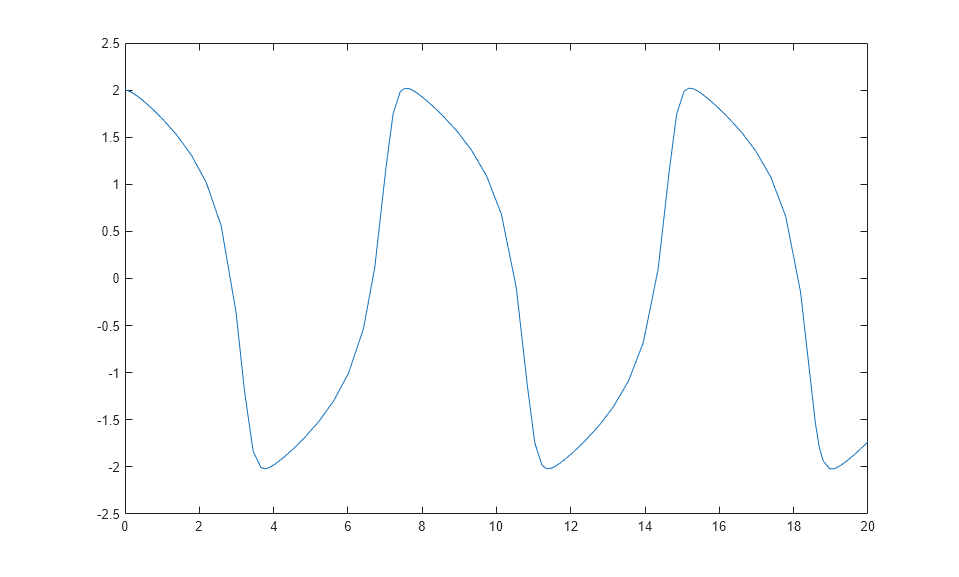
You can also plot the data from the workspace in a MATLAB figure. For example, plot the x1 signal.

x1_data = out.ScopeData{1}.Values.Data(:,1); x1_time = out.ScopeData{1}.Values.Time; plot(x1_time,x1_data)

Pause Display While Running

Use the Snapshot button to pause the scope display while the simulation keeps running in the background.

1. Open a scope window and start the simulation.
2. Select > .
   
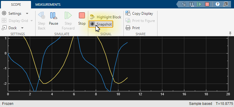
   The scope window status in the bottom left is frozen, but the simulation continues to run in the background.
3. Interact with the paused display. For example, use measurements, copy the scope image, or zoom in or out.
4. To unfreeze the display, select > again.

Copy Scope Image

You can copy and paste a scope image into a document.

1. Open the scope window and run the simulation.
2. Select > .
   
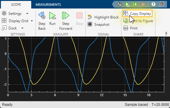
3. Paste the image into a document.
   
   By default, saves a printer-friendly version of the scope with a white background and visible lines. If you want to paste the exact scope plot displayed, select > . Then, under Axes Style, select .

Modify _x_-axis of Scope

This example shows how to modify the _x_-axis values of the Scope block using the Time span and Time display offset parameters. The Time span parameter modifies how much of the simulation time is shown and offsets the _x_-axis labels. The Time display offset parameter modifies the labels used on the _x_-axis.

You can also use this procedure for the Time Scope block, Floating Scope block, or Scope viewer.

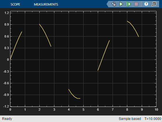
Open the model and run the simulation to see the original scope output. The simulation runs for 10 time steps, stepping up by one at each time step.

model = "ModifyScopeXAxis"; sim(model);

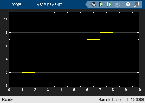
Modify Time Span Shown

Change the time span shown in the scope to 2. In the scope window, select Scope > Settings. Then, under Time, set Time span to 2.

Alternatively, you can set the time span of the scope programmatically.

scopeConfig = get_param(model+"/Scope","ScopeConfiguration"); scopeConfig.TimeSpan = "2"; sim(model);

The _x_-axis of the scope now shows only the last two time steps and offsets the _x_-axis labels to show 0 to 2. The bottom toolbar shows that the _x_-axis is offset by 8. This offset is different from the Time display offset value.

The Time span parameter is useful if you do not want to visualize signal initialization or other startup tasks at the beginning of a simulation.

Offset _x_-axis Labels

Change labels on the _x_-axis to show values between 5 and 7. Select Scope > Settings. Then, under Time, set Time display offset to 5.

Alternatively, you can change the displayed _x_-axis labels programmatically.

scopeConfig.TimeDisplayOffset = "5"; sim(model);

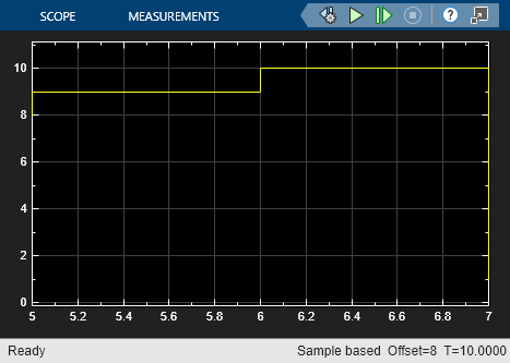
Now, the same time span of 2 is shown in the scope, but the _x_-axis labels are offset by 5, starting at 5 and ending at 7.

Select Number of Displays and Layout

1. From a Scope window, select > .
2. Select the number of displays and the layout you want. You can select up to a 5-by-5 grid.
   
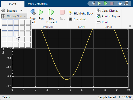
3. Click to apply the selected layout to the Scope window.

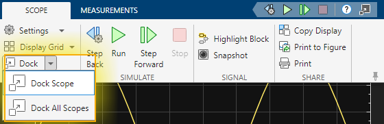
Dock and Undock Scope Window to MATLAB Desktop

To dock a scope:

1. In the scope window, select the tab.
2. To dock the scope, click Dock. You can also clickDock Scope from the drop-down menu to dock an individual scope. To dock all opened scopes, select Dock All Scopes.
   
   When a scope is docked, the scope window is placed in the scope container. The scope container is a single window that you can use to dock multiple scope windows of a Simulink model.

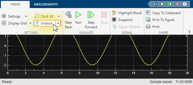
To undock a scope:

1. In the scope container, select the Home tab.
2. Click Undock.
   

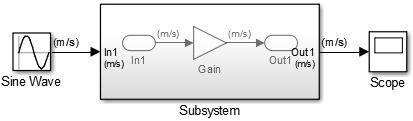
Show Signal Units on Scope Display

You can specify signal units at a model component boundary (Subsystem and Model blocks) using Inport and Outport blocks. See Unit Specification in Simulink Models. You can then connect a Scope block to an Outport block or a signal originating from an Outport block. In this example, the Unit property for the Out1 block is set to m/s.

Show Units on Scope Display

1. From the Scope window toolbar, select > .
2. Under Y-axis, in the Y-axis label box, enter a title for the _y_-axis followed by (%<SignalUnits>). For example, typeVelocity (%<SignalUnits>).
   Signal units display on the _y_-axis label as meters per second (m/s). The scope also displays units when you pause on a data cursor.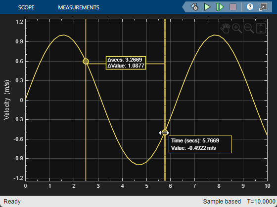
   

Show Units on Scope Display Programmatically

1. Get the scope properties. In the Command Window, enter this command.
   load_system("my_model")
   s = get_param("my_model/Scope","ScopeConfiguration");
2. Add a _y_-axis label to the first display.
   s.ActiveDisplay = 1
   s.YLabel = "Velocity (%)";

You can also set the model parameter ShowPortUnits to'on'. All scopes in your model, with and without(%<SignalUnits>) in the Y-Label property, show units on the displays.

load_system("my_model") get_param("my_model","ShowPortUnits")

set_param("my_model","ShowPortUnits","on")

Determine Units from Logged Data Object

When saving simulation data from a scope with theDataset format, you can find unit information in the logged data object.

Note

Scope support for signal units is only available for theDataset logging format and not for the legacy logging formats Array,Structure, and Structure With Time.

1. Set the Scope block to log data. Select > . Then, under Logging, selectLog data to workspace.
2. Run the simulation.
3. When the model is configured to return results as a single simulation output, scope data is saved as a property of theSimulationOutput object.
   out.ScopeData.getElement(1).Values.DataInfo
   Package: tsdata
   Common Properties:
   Units: m/s (Simulink.SimulationData.Unit)
   Interpolation: linear (tsdata.interpolation)
   When the model is not configured to return results as a single simulation output, scope data is saved as aSimulink.SimulationData.Dataset object.
   ScopeData.getElement(1).Values.DataInfo
   Package: tsdata
   Common Properties:
   Units: m/s (Simulink.SimulationData.Unit)
   Interpolation: linear (tsdata.interpolation)

Connect Signals with Different Units to Scope

When a scope has multiple ports, each port receives data with only one unit. If you try to combine signals with different units, for example, by using a Bus Creator block, the software returns an error.

Scopes show units depending on the number of ports and displays:

• Number of ports equal to the number of displays — One port is assigned to one display with units for the port signal shown on the _y_-axis label.
• Greater than the number of displays — One port is assigned to one display, with the last display assigned the remaining signals. Different units are shown on the last_y_-axis label as a comma-separated list.

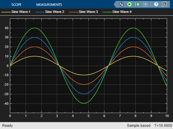
Plot an Array of Signals

This example shows how the scope plots an array of signals.

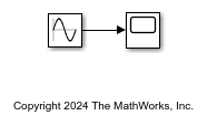
In this simple model, a Sine Wave block is connected to a scope block. The Sine Wave block outputs four signals with the amplitudes [10, 20; 30 40]. The Scope block displays each sine wave in the array separately in the matrix order (1,1), (2,1), (1,2), (2,2).

Scopes in Referenced Models

This example shows the behavior of scopes in referenced models. When you use a scope in a referenced model, information from the model hierarchy can produce different output results than if you run the model containing the scope as a top model.

Note

Scope windows display simulation results for the most recently opened top model. Playback controls in scope blocks and viewers simulate the model containing that block or viewer.

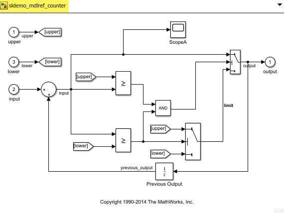
This example uses the sldemo_mdlref_counter model both as a top model and as a referenced model in the sldemo_mdlref_basic model.

Open the model.

openExample("simulink/FindMdlrefsFindReferencedModelsinModelReferenceHierarchyExample","supportingfile","sldemo_mdlref_basic")

Double-click the Model block named CounterA. Thesldemo_mdlref_counter model opens as a referenced model, as you can see in the Explorer Bar.

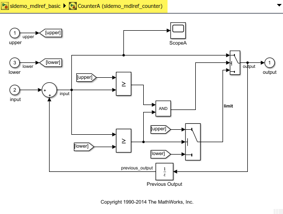
Run the simulation. Then, open the Scope block namedScopeA. The scope visualizes the data from the entire model.

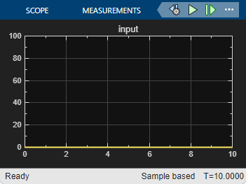
If you specifically want to visualize a referenced model in isolation, open the model as a top model. In the sldemo_mdlref_basic model, right-click theCounterA Modelblock and select . The model opens in another window and the Example Bar shows only thesldemo_mdlref_counter model name.

When you run the simulation from either the Simulink window or the scope window, the scope visualizes the model without any reference to another model. In this case, the model input is zero the entire time.

Scopes Within Enabled Subsystem

When placed within an Enabled Subsystem block, scopes behave differently depending on the simulation mode:

• Normal mode — A scope plots data when the subsystem is enabled. The display plot shows gaps when the subsystem is disabled.
  
• External, accelerator, and rapid accelerator modes — A scope plots data when the subsystem is enabled. The display connects the gaps with straight lines.
  

See Also

Scope | Floating Scope and Scope Viewer

Topics

• Scope Blocks and Scope Viewer Overview
• Floating Scope and Scope Viewer Tasks