Combinatorial algorithms for structural variation detection in high-throughput sequenced genomes (original) (raw)

Abstract

Recent studies show that along with single nucleotide polymorphisms and small indels, larger structural variants among human individuals are common. The Human Genome Structural Variation Project aims to identify and classify deletions, insertions, and inversions (>5 Kbp) in a small number of normal individuals with a fosmid-based paired-end sequencing approach using traditional sequencing technologies. The realization of new ultra-high-throughput sequencing platforms now makes it feasible to detect the full spectrum of genomic variation among many individual genomes, including cancer patients and others suffering from diseases of genomic origin. Unfortunately, existing algorithms for identifying structural variation (SV) among individuals have not been designed to handle the short read lengths and the errors implied by the “next-gen” sequencing (NGS) technologies. In this paper, we give combinatorial formulations for the SV detection between a reference genome sequence and a next-gen-based, paired-end, whole genome shotgun-sequenced individual. We describe efficient algorithms for each of the formulations we give, which all turn out to be fast and quite reliable; they are also applicable to all next-gen sequencing methods (Illumina, 454 Life Sciences [Roche], ABI SOLiD, etc.) and traditional capillary sequencing technology. We apply our algorithms to identify SV among individual genomes very recently sequenced by Illumina technology.

Recent introduction of the next-generation sequencing technologies has significantly changed how genomics research is conducted (Mardis 2008). High-throughput, low-cost sequencing technologies such as pyrosequencing (454 Life Sciences [Roche]), sequencing-by-synthesis (Illumina and Helicos), and sequencing-by-ligation (ABI SOLiD) methods produce shorter reads than the traditional capillary sequencing, but they also increase the redundancy by 10- to 100-fold or more (Shendure et al. 2004; Mardis 2008). With the arrival of these new sequencing technologies, along with the capability of sequencing paired-ends (or “matepairs”) of a clone insert that follows a tight length distribution (Raphael et al. 2003; Volik et al. 2003; Dew et al. 2005; Tuzun et al. 2005; Korbel et al. 2007; Bashir et al. 2008; Kidd et al. 2008; Lee et al. 2008), it is becoming feasible to perform detailed and comprehensive genome variation and rearrangement studies.

The genetic variation among human individuals has been traditionally analyzed at the single nucleotide polymorphism (SNP) level as demonstrated by the HapMap Project (International HapMap Consortium 2003, 2005), where the genomes of 270 individuals were systematically genotyped for 3.1 million SNPs. However, human genetic variation extends beyond SNPs. The Human Genome Structural Variation Project (Eichler et al. 2007) has been initiated to identify and catalog structural variation (SV). In the broadest sense, SV can be defined as the genomic changes among individuals that are not single nucleotide variants (Tuzun et al. 2005; Eichler et al. 2007). These include insertions, deletions, duplications, inversions, and translocations (Feuk et al. 2006; Sharp et al. 2006) (see Supplemental material for details on types of SV).

End-sequence profiling (ESP) was first presented by Volik et al. (2003) and Raphael et al. (2003) to discover SV events using bacterial artificial chromosome (BAC) end sequences to map structural rearrangements in cancer cell line genomes, and it was used by Tuzun et al. (2005) to systematically discover structural variants in the genome of a human individual. Several other genome-wide studies (Iafrate et al. 2004; Sebat et al. 2004; Redon et al. 2006; Cooper et al. 2007; Korbel et al. 2007) demonstrated that SV among normal individuals is common and ubiquitous. More recently, Kidd et al. (2008) detected, experimentally validated, and sequenced SV from eight different individuals. The ESP method was also utilized by Dew et al. (2005) to evaluate and compare assemblies and detect assembly breakpoints.

As the promise of these next-generation sequencing (NGS) technologies became reality with the publication of the first three human genomes sequenced with NGS platforms (Bentley et al. 2008; Wang et al. 2008; Wheeler et al. 2008), the sequencing of more than 1000 individuals (http://www.1000genomes.org), computational methods for analyzing and managing the massive numbers of the short-read pairs produced by these platforms are urgently needed to effectively detect SNPs, SVs, and copy-number variants (Pop and Salzberg 2008). Since most SV events are found in the duplicated regions (Eichler et al. 2007; Kidd et al. 2008), the algorithms must also be able to discover variation in the repetitive regions of the human genome.

Detection of SVs in the human genome using NGS technologies was first presented by Korbel et al. (2007). In this study, paired-end sequences generated with the 454 Life Sciences (Roche) platform were employed to detect SVs in two human individuals; however, the same algorithms and heuristics designed for capillary-based sequencing presented by Tuzun et al. (2005) were used, and no further optimizations for NGS were introduced. Campbell et al. (2008) employed Illumina sequencing to discover genome rearrangements in cancer cell lines; however, they considered one “best” paired map location per insert, by the use of the alignment tool MAQ (Li et al. 2008), and thus did not utilize the full information produced by high-throughput sequencing methods. In the first study on the genome sequenced with a NGS platform (Illumina) that produced paired-end sequences, Bentley et al. (2008) also detected SVs using the same methods and unique map locations of the sequenced reads.

More recently, Lee et al. (2008) presented a probabilistic method for detecting SV. In this work, a scoring function for each SV was defined as a weighted sum of (1) sequence similarity, (2) length of SV, and (3) the square of the number of paired-end reads supporting the SV. The scoring function was computed via a hill-climbing strategy to assign paired-end reads to SVs. In theory, the method of Lee et al. (2008) can be applied to data generated by new sequencing technologies; however, the experiments presented in this work were based on capillary sequencing (Levy et al. 2007). In another study, Bashir et al. (2008) presented a computational framework to evaluate the use of paired-end sequences to detect genome rearrangements and fusion genes in cancer; note that no NGS data were utilized in this study due to lack of availability of sequences at the time of publication.

In this paper, we present novel combinatorial algorithms for SV detection using the paired-end, NGS methods. In comparison to “naïve” methods for SV detection, our algorithms evaluate all potential mapping locations of each paired-end read and decide on the final mapping and the SVs they imply interdependently. We define two alternative formulations for the problem of computationally predicting the SV between a reference genome sequence (i.e., human genome assembly) and a set of paired-end reads from a whole genome shotgun (WGS) sequence library obtained via an NGS method from an individual genome sequence. The first formulation, which aims to obtain the most parsimonious mapping of paired-end reads to the potential structural variants, is called Maximum Parsimony Structural Variation Problem (MPSV). MPSV problem turns out to be NP-hard; we give a simple O(log n) approximation algorithm to solve this problem in polynomial time. This algorithm is based on the classical approximation algorithm to solve the “Set-Cover” problem from the combinatorial algorithms literature and thus is called the VariationHunter-Set Cover method (abbreviated VariationHunter-SC). The second formulation aims to calculate the probability of each SV. For this variant we give expressions for (1) the probability of each possible SV conditioned on other SVs and the paired-end reads that “support them,” and (2) the probability of mapping each paired-end read to a particular location, conditioned on the set of SVs that are “realized.” We show how to obtain a consistent set of solutions to these expressions iteratively. The resulting algorithm is called VariationHunter-Probabilistic (VariationHunter-Pr). We test our algorithms (VariationHunter-SC and VariationHunter-Pr) on a paired-end WGS library generated with Illumina technology and compare the results with the validated SV set from the genome of the same individual, obtained via fosmid-based capillary end-sequencing (Kidd et al. 2008). We compare our results with the SV calls reported earlier on the same data set (Bentley et al. 2008), which was based on mapping each paired-end read to a single location (with the minimum number of mismatches) and clustering the mappings greedily to obtain the SVs.

Methods

A general method for using paired-end long reads to detect SVs between the new donor genome and reference genome was first introduced by Volik et al. (2003) and Tuzun et al. (2005). This general strategy is based on aligning the paired-end sequenced reads to the reference genome and observing significant differences between the distance of matepairs6 when mapped to the reference genome and their expected distance, which indicates a deletion or an insertion event. Furthermore, one can also deduce inversion events: If one of the two ends of a pair has a “wrong” orientation, this is likely a result of an inversion (Tuzun et al. 2005). In case the two ends are everted, i.e., both ends of a paired-end have reverse orientation (with respect to each other) but their order is preserved in the reference genome, it is likely to have a tandem repeat. Finally, paired-end reads mapping to two different chromosomes are likely to result from a transchromosomal event (see Supplemental material).

At the core of the above general strategy is the computation of the expected distance between matepairs in the donor genome, which is referred to as insert size (InsSize). Previous works (Tuzun et al. 2005; Korbel et al. 2007; Lee et al. 2008) assume that for all paired ends, InsSize is in some range [_minLen, maxLen_], which can be calculated as described by Tuzun et al. (2005).

An alignment of a paired-end read to reference genome is called concordant (Tuzun et al. 2005), if the distance between aligned ends of a pair in the reference genome is in the range [_minLen, maxLen_], and both the orientation and the chromosome the paired-end read is aligned to are “correct.” For instance, in the Illumina platform (for other platforms it might be different), a paired-end read is considered to be aligned in the “correct” orientation if the left matepair is mapped to the “+” strand (which is represented by +), and the right mate pair is mapped to the “−” strand (which is represented by −). A paired-end read that has no concordant alignment in the reference genome (Tuzun et al. 2005; Korbel et al. 2007; Lee et al. 2008) is called a discordant paired-end read (which indicates a possibility of a SV; see Supplemental material).

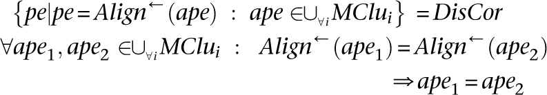
Let the set of discordant paired-end reads be represented as DisCor = {_pe_1, _pe_2, …, pen}. Each of these discordant matepairs can have multiple (pairs of) locations in genome that they can be aligned to with high sequence similarity (e.g., ≥90%7), which can be represented by Align(pei) = {a_1_pei, a_2_pei,…, ajpei}. We also define Align←(ajpei) = pei.

Note that each alignment location in the reference genome (as mentioned above, all alignments of paired-end reads to the reference genome require a sequence similarity >90%), ajpei, includes a triplet of a pair of loci in the genome and orientation of the mapping.

More specifically, ajpei = (pei, l(ajpei), r(ajpei), or(ajpei)), where l(ajpei) is the end locus of the left end, r(ajpei) is the start locus of the right end, and or(ajpei) is the orientation of the mapping (or(ajpei) = +− is the orientation representing no inversion, or(ajpei) = ++ shows an inversion event where the right matepair is in the inverted region, and or(ajpei) = −− represents the fact that the left matepair is in the inverted region).

Our algorithm(s) will obtain a unique alignment Map(pei) from the set Align(pei) for each paired-end read pei. We denote this by Mapcorr(pei), the “correct” location for the paired-end read pei. The goal of our algorithm(s) is to pick Map(pei) = Mapcorr(pei).

We represent a SV event by SV (t, PosL, PosR, Ranmin, Ranmax) (abbreviated SV), which represents a SV of type t ∈ {Ins, Del, Inv}8 that is located between positions PosL and PosR of the reference genome, and the length of SV is between ranges Ranmin and Ranmax. All SVs have breakpoints, and it is desirable to find these breakpoints; however, using the information of paired-end reads, we can only deduce a range for the location of these breakpoints (e.g., if there is a single mapping for a particular paired-end read that supports a deletion, which is supported only by this paired-end, it is unclear what is the exact size of deletion or the exact locations of the breakpoints).

An alignment of discordant paired-end read ape is said to be supporting a SV (t, PosL, PosR, Ranmin, Ranmax) when:

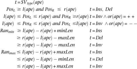
Here, SVtype(ape) represents the SV type ape supports as a consequence of the distance and orientation of its ends.9

A set of alignment of discordant paired-end reads that can support the same potential SV is called a “valid cluster” and is denoted by

Thus, a valid cluster is a set of alignments of discordant paired-end reads that support a particular SV. A set of discordant mappings forms a valid cluster if it satisfies a set of rules, based on the type of SV it supports as follows (in the following rules, InsLen, DelLen, and InvLen represent the possible length of SVs of type insertion, deletion, and inversion, respectively, supported by valid cluster Clu).

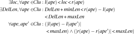
Insertion: A set of discordant alignments, Clu, is a valid cluster that supports an “insertion” if

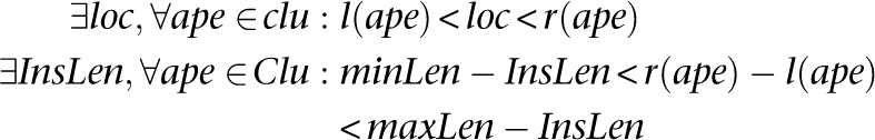
Deletion: A set of discordant alignments, Clu, is a valid cluster that supports a “deletion” if

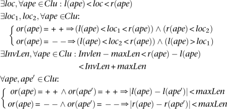
Inversion: A set of discordant alignments, Clu, is a valid cluster that supports an “inversion.” We focus only on inversions with size at least twice the size of insert size (InsSize) of the paired-end reads; this is the most common scenario. The formulae to capture all the inversions are much more complex and probably not very reliable.

A “valid” cluster VClui is said to be supporting a SV event SV if all the mappings in VClui support the structural variation SV. An alignment of paired-end read, such as ape, is said to be “materialized” by the algorithm if it maps the paired-end read, _Align_←(ape), to alignment ape. A valid cluster is said to be “materialized” (by the algorithm) if for each j, 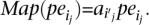We denote materialized clusters as MCluj.

SV detection based on maximum parsimony

The Maximum Parsimony Structural Variation (MPSV) problem asks to compute a unique mapping for each discordant paired-end read in the reference genome such that the total number of implied SVs is minimized. The minimum number of SVs implied by the mappings is the most parsimonious one under the implicit assumption that all SVs are equally likely.10 We will consider varying probabilities for each SV type, length, and support by number of paired-end reads supporting it, and sequence similarity in the description and the solution of the probability-based problem. Note that for the MPSV problem, we provide an algorithm with an approximation guarantee.

More formally, the MPSV problem asks to compute the minimum number of materialized clusters (sets) MClui given a set of DisCor paired-end reads and a set alignment locations (Align(pei)) for each paired-end pei such that

The MPSV problem can be further constrained (Tuzun et al. 2005; Korbel et al. 2007; Lee et al. 2008) so that each materialized cluster includes at least two reads. The problem can also be generalized, in a way that each SV has an associated cost, which may be based on the sequence similarity in the alignments, the number of pair-ends supporting it, and length of SV. We prove that the MPSV problem is NP-hard using a simple reduction from the well-known set cover problem (see Supplemental material). As a result, we describe an approximation algorithm to the MPSV problem that runs in polynomial time.

Before proceeding with the approximation algorithm for the MPSV problem, we have to introduce the notion of a “maximal valid cluster”: A maximal valid cluster is a valid cluster for which no valid superset exists. For each type of SV, the maximal valid clusters can be computed in polynomial time as follows:

1. Given the complete set of paired-end read alignments, let Ij,i be an “interval” on the genome sequence that corresponds to the paired-end read alignment ajpei; let Ij,i = [l(ajpei), r(ajpei)]. On this set of intervals, compute the complete collection of maximal interval sets in which every interval intersects with every other interval. Denote by MPos = {_MPos_1, · · ·, MPosp} the collection of these maximal interval sets. Let MPos can be computed greedily in time polynomial with the number of intervals: Scan the intervals from “left” to “right,” adding to _MPos_1 each interval that intersects with all intervals added to _MPos_1 so far. Start _MPos_2 by including all members of _MPos_1, excluding the one that has the leftmost right end and iterate. At each step i, eliminate each MPosi if it ends up to be a proper subset of MPosi − 1.
2. This step is only necessary for detecting inversions: For each maximal interval MPosi (which is representing an inversion), create all the subsets of MPosi (denoted by such that
   
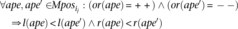
   These subsets can be created simply in polynomial time as follow. First, consider the genome interval that MPosi covers (i.e., Interval = [min(l(ape)), max(r(ape))]).
   Second ∀x, y ∈ Interval: x < y create a new set such that:
   
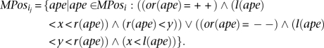
   Finally, remove any set that is a proper subset of another such set. It is easy to see that the total number of such sets is O(|MPosi|2).
3. For each paired-end read alignment in MPosi (or for inversions) and for each SV type, consider the implied range of the length of this SV. Find the maximal subsets of Mposi (or for inversions) in which the ranges (for a particular SV type) of all paired-end read alignments intersect. Again, by the simple greedy algorithm described for the previous step, this can be done in time polynomial with the size of MPosi (or for inversions).
4. Consider the collection of the maximal subsets of paired-end read alignments obtained above. First, filter out any maximal subset that is contained in another (it is easy to see that the remaining sets are indeed all of the maximal valid clusters). Then, simply apply the well-known greedy algorithm for the approximate set cover problem (described below) on these maximal subsets to obtain the set of SV.

Given a set U = {_e_1,…, en} and a collection of subsets of U, S = {_S_1, _S_2,…, Sm}, the set cover problem asks to find the smallest subset of S whose union includes each ei ∈ U. The greedy algorithm, which, at each iteration, picks up the set that includes the maximum number of uncovered elements of U until all elements of U are covered, provides an O(log n) approximation to the optimal solution (an interested reader can find a proof in Vazirani [2001]). Interestingly enough, this simple algorithm implies an approximation factor of O(log n) for the MPSV problem after the following modification: In each iteration of the algorithm, pick up the maximal paired-end read alignment set with the maximum number of uncovered paired-end reads (the proof for the approximation factor trivially follows the proof for the set cover problem [Vazirani 2001]). We have named this algorithm VariationHunter-Set Cover (abbreviated VariationHunter-SC), because of its use of the original set cover algorithm.

In our experiments we also consider a weighted version of the VariationHunter-SC method. Here, each set (i.e., maximal valid cluster) has a weight associated with it, which is a summation of the weights associated with each paired-end read mapping. The weight of a paired-end mapping, on the other hand, is based on the alignment score (between the paired-end read and the mapping location).

A probabilistic model for capturing SV and paired-end read alignments

The MPSV problem as described above aims to map each paired-end read to a particular SV with the goal of minimizing the number of SVs they collectively imply. This formulation implicitly assumes that each SV occurs independently—dependencies between SVs are ignored. Consider now the following scenarios supported by a given set of paired-end reads: (1) all (discordant) paired-end reads are mapped to only two locations (supporting two SVs), one with very high support and the other with significantly low support; (2) the paired-end reads are mapped to three locations supporting three SVs, all with roughly equal support. The joint probability of the SVs implied by scenario (1) may be much lower than that implied by scenario (2).11

As a result, it is highly desirable to compute (at least approximately) the probability for each potential SV given the potential mappings of all paired-end reads. Once these probabilities are computed, it may become possible to determine the set of SVs that is most likely to be implied by the paired-end reads we have.

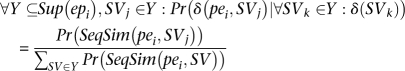
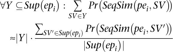
In what follows, we show how to compute the probability of each SV, given the mappings of all input paired-end reads and the probability of a particular alignment of a paired-end read, given all SVs. We have called this method, which calculates the probability of each SV, VariationHunter-Probability (abbreviated VariationHunter-Pr). First, we will define a few sets and variables that will be used through the rest of the paper. Let set SSV be the set of all potential SVs that have at least one paired-end supporting them. Set Sup(pei) is a subset of set SSV, such that each potential SV is a member of Sup(pei) if there exists an alignment of paired-end pei that supports it. More formally, Sup(epi) = {SV|SV ∈ SSV, ∃ape ∈ Align(pei): ape supports SV}. Let SeqSim(pei, SVj) be the sequence similarity score of the alignment of paired-end pei that supports SVj (if a paired-end pei does not have any alignments that support SVj, then SeqSim(pei, SVj) = 0); also, Pr(SeqSim(pei, SVj)) is the probability of paired-end pei supporting SVj solely based on sequence similarity score SeqSim(pei, SVj).

Let δ (SVj) be the indicator variable for potential structural variation SVj (i.e., δ (SVj) = 1 iff SVj is “correct”). We also would define δ (pei, SVj) as the indicator variable that paired-end pei if mapped to “correct” location supports the structural variations SVj (i.e., δ (pei, SVj) = 1 iff the correct location of mapping of pei supports SVj).

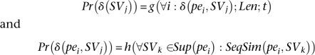
We claim that Pr(δ (SVj)) is a function of δ (pei, SVj) for all pei, length, and type of the SV. In addition, Pr(δ (pei, SVj)) is a function of all the SVs that paired-end pei potentially can support and the sequence similarity of the paired-end pei and the alignments that support SVj. Formally speaking, we will have two sets of equations:

Note that a discordant paired-end read that supports only one potential SV in the reference genome may not indicate a SV: In certain cases, insert size errors can be responsible for the deviation in the paired-end read length.12 Obviously, the more paired-end reads support a potential SV, the less the chance is that the deviation in read length is due to a read error. Furthermore, the longer the potential SV is, the lower the chance we have that a read error is responsible for the deviation in read length.

The probability of SVs based on mappings of paired-end reads function

In this section, we give expressions for the probability of a given SVj conditioned on the (correct) mappings of paired-end reads. Let f(t; Len; k) be the probability of a SV of type t and length Len, when supported exactly by k paired-end reads when all the reads are mapped to correct location.

The value of f should increase with k and decrease with Len.13 Although the length of a SV implied by one or more mappings can only be obtained within a range, we will simply use 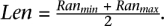.Assuming that set A is set of paired-end reads that (when mapped to correct location) support SVj, we have:

Now we are ready to give the equation for Pr(δ (SVj)):

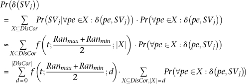
Furthermore, assuming independence between mappings of different paired-end reads14

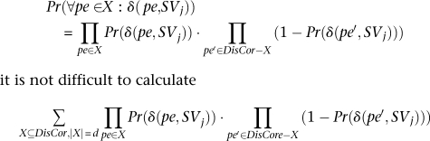
it is not difficult to calculate

which is the probability of exactly d paired-end reads from set DisCor when mapped to correct location support SVj, through dynamic programming. Let Pr(i, m), be the probability of exactly i paired-end reads supporting SVj among the first m paired-end reads in set DisCor (when paired-end reads in DisCor are mapped to the correct locations)

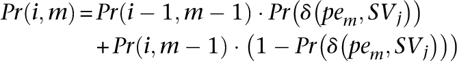
As can been seen, the above recursive equation can be calculated using Dynamic Programming given Pr(δ (_pe_m, _SV_j)) for all j and m.

The probability of paired-end read mappings based on SV

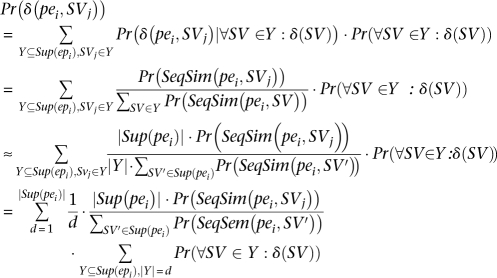
In this section, we will give the formulation that we use to calculate probability of a paired-end pei supporting a potential structural variation SVj.

Given a paired-end read pei and potential structural variation SVj, we have:

We use the fact that

Now we can calculate pr (δ (pei, SVj)) as:

It is clear that can be calculated using a similar dynamic programming method used in the section “The probability of SVs based on mappings of paired-end reads function,” assuming independence between different potential SVs.

Identification of the most probable set of SVs

It is not difficult to compute solutions to the expressions we gave above for the probabilities of the SVs and paired-end read mappings iteratively. Initially, we assume that each of the potential SVs is equally probable. The set of SVs implied by the maximal valid clusters (as defined in the section “SV detection based on maximum parsimony”) can act as the potential SVs. In iteration i, calculate the probability of each mapping (or paired-end reads), considering the probabilities of SVs from iteration i − 1, and then calculate the probability of each SV, based on the probabilities of paired-end reads from iteration i. The iterative procedure terminates once the total difference in the probabilities of the SVs and mappings in iteration i and iteration i − 1 is within a factor of ε. Finally, we can select the SVs with probability above a user-defined cut-off (which will be set to 0.9 in the remainder of the paper).

Results and Discussion

We tested our algorithms with the paired-end read WGS library generated from the genome of an anonymous donor (NA18507) using the Illumina technology (Bentley et al. 2008). We first downloaded ∼3.5 billion end sequences (∼1.75 billion matepairs), each of length 36 − 41 bp and insert size 200 bp—the reads are available at the NCBI Short Read Archive.15 This constitutes ∼42× sequence and ∼120× physical coverage of the complete genome sequence. A large set of SV events in this individual genome sequence was previously detected and experimentally validated using longer inserts (i.e., 40-Kbp fosmids) by Kidd et al. (2008). We used this data set to test the accuracy of our algorithms and compare them with that of the method used by Bentley et al. (2008) (Table 1). Note that we do not compare our algorithms with the method presented by Lee et al. (2008), as the current implementation of this method cannot handle NGS data in the scale studied here (S Lee, pers. commun.).

Table 1.

Comparison of SV detected in the Illumina paired-end read library generated from the genome of NA18507 with the validated sites of variation using a fosmid-based approach from the same individual

Due to the lower sequence quality generated by the Illumina platform, we first pre-screened the paired-end reads as follows:

• (1) We removed any matepairs from consideration if one (or both) of the end sequences had an average phred (Ewing and Green 1998) quality value <20. This resulted in the removal of ∼1.3 billion reads, leaving us with ∼2.2 billion reads.
• (2) Approximately 50 million pairs of sequences were first sampled and mapped to the reference genome to establish length distribution statistics. The average span length turned out to be 209 bp and the standard deviation (std) was 13.4 bp (see Supplemental material for detailed length distribution figures).
• (3) All ∼2.2 billion end sequences were then mapped to the reference genome using our in-house sequence mapping tool mrFAST (http://eichlerlab.gs.washington.edu/mrfast/), and all possible locations within an edit distance of two were considered.16 Out of ∼2.2 billion reads, 2.17 billion of them (95.9% of the total) were mapped to the reference genome successfully. The remainder were eliminated. The 2.17 billion reads that were mapped corresponded to (1) ∼804 million paired-end reads for which both ends were mapped (yielding ∼56× physical coverage), and (2) 562 billion “one-end” anchors, i.e., paired-end reads where only one end was mapped.
• (4) We then discarded any matepairs where the total number of paired configurations exceed 1000, or if either of the end sequences mapped to more than 5000 locations. The read mapping stage was completed within a week using 200 CPU cores on our computational cluster. (Further details on the map statistics are provided in the Supplemental material.)

As per earlier work (Tuzun et al. 2005; Korbel et al. 2007; Kidd et al. 2008; Lee et al. 2008), we call a clone insert concordant if it spans within 4× std of the average length (i.e., 155–266 bp for this data set), and the mapping orientations of both ends obey the rules dictated by the WGS library.17 In the end, we obtained 787,667,370 concordant and 16,766,282 discordant pairs (296,408,665 discordant combinations), each indicating a deletion, insertion, inversion, or translocation event, or everted pairs. All concordant pairs were then removed from further consideration.18

We used both VariationHunter-SC and VariationHunter-Pr algorithms to analyze the map locations of the discordant paired-end read sequences obtained as per above. On a single standard PC, the VariationHunter-SC algorithm completed the analysis in <1 h; VariationHunter-Pr required ∼3 h for the same task.

Before reporting SVs, we applied a number of postprocessing steps:

• (1.a) In order to increase our confidence in SV prediction by the unweighted VariationHunter-SC, we filtered out variants that were supported by at most five unique paired-end reads.
• (1.b) In the case of the weighted VariationHunter-SC, we filtered out variants with total support of at most three (the total support of an SV is the sum of weights of unique paired-end reads supporting the SV). Note that two paired-end reads supporting a SV is considered unique if there is at least 5 bp between the start coordinates of their map locations (Tuzun et al. 2005; Kidd et al. 2008).
• (2) Another problem that we had to tackle was the elimination of contradictory SV predictions that imply more than two alleles. For that purpose we considered all clusters of SVs that overlapped: Among the SVs in a cluster, we filtered out those with the smallest paired-end read support. In case two SVs had the same support, we filtered out the one that was shorter.
• (3) We filtered out all deletions that were >500 Kb and inversions that were longer than 10 Mb.

After the completion of the final postprocessing step, the weighted VariationHunter-SC algorithm returned a total of 8959 deletions, 504 inversions, and 5575 insertions, while its unweighted version returned a total of 7599 deletions, 433 inversions, and 3772 insertions. In contrast, the VariationHunter-Pr algorithm predicted 8537 deletions, 181 inversions, and 7142 insertions, each with probability ≥90%.

We compared the predicted deletions and inversions with both sample-level and locus-level validated sites of variation in Table 1. Structural variants detected by the fosmid ESP approach that are validated using the fosmids from the same individual are categorized as “sample-level validated.” If a variant is predicted in multiple individuals (including NA18507), but validated with fosmids from another individual (to reduce cost and labor for validating common variants), then it is categorized as “locus-level validated.”

Our thresholds for calling a predicted deletion correct are stricter than that used in the original Illumina study (Bentley et al. 2008): We require at least 50% reciprocal overlap between the deletion intervals. We consider a predicted inversion correct if it has some overlap with a validated inversion. Based on these premises, we provide a three-way comparison for the deletions predicted by VariationHunter-SC (both weighted and unweighted versions), VariationHunter-Pr, and the method of Bentley et al. (2008) (see Supplemental material for details).

In total, we were able to predict ∼62% of the validated deletions with the weighted VariationHunter-SC algorithm, whereas the method of Bentley et al. (2008) can capture only ∼53% of the validated deletions, provided the same overlap thresholds are applied to both methods as explained above. Our true positive rate can be improved to 64/92 (70%) for sample-level validated sites, and 96/143 (67%) for locus-level validated sites, by simply removing the minimum weighted support requirement; however, this also increases the total number of predicted deletions to 13,320 (with a total length of 134 Mbp) as opposed to 8959 deletions (with a total length of 23.4 Mbp).

Note that it is only possible to capture insertion events with a length upper-bounded by the difference between the average insert size and the total paired-end read length (i.e., 209 − 72 = 137 bp for this set) using paired-end reads without the use of sequence assembly methods. Since the average length of a fosmid clone is much bigger, i.e., 40 Kbp, Kidd et al. (2008) reported insertions of 800 bp–8 Kbp in size; thus, our insertion predictions cannot be compared with the insertion events reported by Kidd et al.

Although the number of deletions we predicted using the Illumina WGS set is significantly higher than the number of validated sites, 24.5% of the predicted intervals we report are ≤100 bp, and 96.75% of the intervals are <8 Kbp (Fig. 1). These deletions were not the focus of the paired-end read analysis provided by Kidd et al. (2008); however, it is possible to test the validity of some of the short indels (≤100 bp) we predicted with another resource presented by Kidd et al. (2008), called deletion/insertion polymorphisms (DIPs). DIPs are indels of length <100 bp and can be detected from the alignment of each capillary sequencing-based read (average length ∼800 bp) to the genome. Two hundred thirty-three of 2200 deletions of length ≤100bp and 135 of 5575 insertions predicted by the weighted VariationHunter-SC algorithm intersect with the DIP database obtained by Kidd et al. (2008) (Table 2). Note that since the sequence coverage of the fosmid end-sequence library used by Kidd et al. (2008) is only 0.3×, the DIP database mentioned above is far from being complete.

Figure 1.

Deletion length histogram of detected SVs from NA18507 in human genome build 36 with the weighted VariationHunter-SC algorithm (weighted_ support ≥ 3). Increased numbers of predicted deletions of size 300 bp and 6 Kbp (due to _Alu_Y and L1Hs repeat units, respectively) are clearly seen in the histogram, confirming the known copy-number polymorphism in retrotransposons (Batzer et al. 1996; Boissinot et al. 2000).

Table 2.

Comparison of small indels (≤100bp) detected in the Illumina paired-end read library generated from the genome of NA18507 with the DIP sites predicted by fosmid end-sequence mapping (Kidd et al. 2008) from the same individual

An investigation of the length distribution of deletions (Fig. 1) will reveal that a significant number of predicted deletions have lengths ∼300 bp and ∼6 Kbp. These figures correspond to the known copy number polymorphism of retrotransposons (Batzer et al. 1996; Boissinot et al. 2000). In addition, the length distribution of deletions with length >100 bp predicted by the weighted VariationHunter-SC algorithm in the genome of NA18507 is similar to the previously reported length distribution of the deletions reported in the Venter genome (Fig. 2; Levy et al. 2007).

Figure 2.

Comparison of deletion size distributions detected from the genome of NA18507 with the VariationHunter-SC algorithm and from Venter genome as reported in Levy et al. (2007).

As a final experimental study, we performed a number of simulations to test the sensitivity and specificity of our algorithms. We first imposed the set of insertions and deletions in chromosomes 1 and 22 reported in the Venter genome (Levy et al. 2007) to the human genome reference assembly build 36. We then added random SNPs independently at each locus with a rate of 0.1% per base. Finally, we randomly generated paired-end sequences from the simulated chromosome sequences (read length 36 bp and span size of 155–264 bp) with estimated 20× sequence coverage. The simulated reads were then mapped to human genome reference assembly build 36 with mrFAST, and the structural variants were predicted by both weighted VariationHunter-SC and VariationHunter-Pr algorithms.

The VariationHunter-SC method captured ∼64% of deletions (>200 bp) in chromosome 1 and 55% of the deletions (size >200 bp) in chromosome 22. 90% of the deletions predicted by VariationHunter-SC were among the simulated deletions (10% false positive rate for both chromosomes). The VariationHunter-Pr had higher recall and was able to capture slightly more deletions (of size >200 bp): 67% in chromosome 1 and 60% for chromosome 22; however, it also returned slightly more false positives (∼13%) for both chromosomes.

In terms of insertions, the VariationHunter-SC method recalled ∼50% of insertions of size 50–80 bp, and VariationHunter-Pr was able to capture 55% of such insertions. The false positive rates were ∼22% and ∼30% for VariationHunter-SC and VariationHunter-Pr, respectively.

The simulation results are very promising especially for deletions; however, we believe that it is possible to improve the predictive power of our methods. Most of the false negatives were due to the short read length and the repetitive nature of the human genome. Matepairs encompassing a nonrecalled deletion were concordantly mapped to other paralogs of repeats and duplications, resulting in removal of such pairs from consideration for SV detection. Future versions of the VariationHunter algorithms will eliminate concordant mappings more carefully for improving SV prediction accuracy in repetitive regions of the human genome.

Conclusion

The algorithms presented in this paper for detecting SVs using new sequencing platforms are shown to be efficient and reliable. However, we have to also point out that although the physical coverage of the Illumina WGS library we used was significantly higher than that of the library used in the fosmid-based approach (Kidd et al. 2008), we still could not recapture some of the validated structural variants (∼30%–38% false negative rate depending on the support threshold). This is likely to be due to mapping artifacts in repeat regions, and sequencing bias associated with Illumina technology such as GC-rich regions. In addition to the mapping issues, there are a number of algorithmic challenges we have to address to improve our algorithms. First, the postprocessing step that filters out the SV predictions that do not have the user-defined matepair support is less than ideal. Sequence coverage with the new sequencing technologies is not uniform in the genome (Bentley et al. 2008; Smith et al. 2008; Wang et al. 2008), and a careful analysis and simulations would be needed to fine-tune the filtering parameters based on the sequence coverage at the predicted SV locus. Another theoretical extension can be made the probabilistic formulation we provide in the section entitled “The probability of SVs based on mappings of paired-end reads function”: The current formulation allows conflicting SVs to occur simultaneously. They are filtered out in another postprocessing step. Ideally, we should be able to address this issue at the time we are calculating the probabilities of SVs by treating potentially conflicting SVs interdependently.

We finally note that the resolution that can be achieved in SV detection using fosmid and Illumina paired-end sequences is quite different. Fosmid-matepair analysis cannot reveal the exact breakpoints of SVs due to larger insert size (40 Kbp) and std (∼3 Kbp); however, smaller insert sizes and tighter length distribution (200 bp and 13 bp, respectively) of the Illumina-based ESP approach, at least in theory, can detect the SV breakpoints within only a few base pairs of error. Therefore, the best data set with which to compare our calls would be the sequenced sites of variation. A select subset of fosmids used in Kidd et al. (2008) is currently being sequenced in full (405 sequenced fosmids were reported in Kidd et al. [2008], unfortunately from a different individual), which will help us discover the exact breakpoints of deletions, insertions, and inversions. Additional experiments are also needed to validate new SV predictions that were not detected by Kidd et al. (2008), which in turn will provide more insight to enhance our algorithms.

Acknowledgments

We thank Jeffrey M. Kidd for discussions on the initial formulations of the SV detection problem, and for providing us with the set of validated structural variants in the NA18507 genome remapped to human reference genome build 36—the original SV set by Kidd et al. (2008) was listed in build 35 coordinates. We also thank Martin Shumway and Mark Ross for technical help in downloading the WGS libraries from the NCBI SRA site, and Tonia Brown for proofreading the manuscript. This work was supported in part by NSERC, Michael Smith Foundation for Health Research, Genome BC grants to S.C.S., and NIH grant HG004120 to E.E.E. E.E.E. is an investigator of the Howard Hughes Medical Institute.

Footnotes

6

Matepairs refer to the two ends of a paired-end read.

7

This is an arbitrary cutoff. Using a higher cutoff value makes the problem easier; however, we might miss some real structural variants.

8

Referring to an insertion, deletion, and inversion, respectively. Note that our methods can be generalized to detect everted pairs and translocation events without much difficulty.

9

Note that there are no range rules for transchromosomal events. Furthermore, although we do not focus on everted paired-end reads or the transchromosomal mappings in this study, our algorithms can be generalized to capture both tandem repeat events and transchromosomal events.

10

Note that minimizing the SVs also will imply that the average number of paired-end reads supporting an SV is maximized—the two goals are equivalent.

11

The reader can easily verify this in the case that the probability of an SV is a linear function of the number of mappings supporting it.

12

By insert size error we mean errors in the distance between the two ends of a read pair by the sequencing platform. For certain platforms, such as Illumina, the probability of such an error is almost nil.

13

Perhaps 1 − f, the probability of a potential read length error, should decrease exponentially with k and linearly with Len.

14

In general, there exists dependency between mapping of different paired-end reads; however, to be able to approximate the values we assume independence between mappings of different paired ends.

16

The reader should also note that our algorithm is compatible with any sequence mapping tool that can return multiple map locations, such as Mosaik (Hillier et al. 2008) or SHRiMP (Yanovsky et al. 2008).

17

For example, in the Illumina platform (short insert library), the upstream end sequence is expected to map to the + strand, where the downstream end sequence is expected to map to the − strand; see the Supplemental material.

18

Note that it is possible to use concordant clones for heterozygosity studies, etc.

[Supplemental material is available online at www.genome.org. The source code of the algorithm implementations and predicted structural variants are available at http://compbio.cs.sfu.ca/strvar.htm.]

References

1. Bashir A, Volik S, Collins C, Bafna V, Raphael BJ. Evaluation of paired-end sequencing strategies for detection of genome rearrangements in cancer. PLoS Comput Biol. 2008;4:e1000051. doi: 10.1371/journal.pcbi.1000051. [DOI] [PMC free article] [PubMed] [Google Scholar]
2. Batzer M, Arcot S, Phinney J, Alegria-Hartman M, Kass D, Milligan S, Kimpton C, Gill P, Hochmeister M, Panayiotis A, et al. Genetic variation of recent Alu insertions in the human populations. J Mol Evol. 1996;42:22–29. doi: 10.1007/BF00163207. [DOI] [PubMed] [Google Scholar]
3. Bentley DR, Balasubramanian S, Swerdlow HP, Smith GP, Milton J, Brown CG, Hall KP, Evers DJ, Barnes CL, Bignell HR, et al. Accurate whole human genome sequencing using reversible terminator chemistry. Nature. 2008;456:53–59. doi: 10.1038/nature07517. [DOI] [PMC free article] [PubMed] [Google Scholar]
4. Boissinot S, Chevret P, Furano AV. L1 (LINE-1) retrotransposon evolution and amplification in recent human history. Mol Biol Evol. 2000;17:915–928. doi: 10.1093/oxfordjournals.molbev.a026372. [DOI] [PubMed] [Google Scholar]
5. Campbell PJ, Stephens PJ, Pleasance ED, O'Meara S, Li H, Santarius T, Stebbings LA, Leroy C, Edkins S, Hardy C, et al. Identification of somatically acquired rearrangements in cancer using genome-wide massively parallel paired-end sequencing. Nat Genet. 2008;40:722–729. doi: 10.1038/ng.128. [DOI] [PMC free article] [PubMed] [Google Scholar]
6. Cooper GM, Nickerson DA, Eichler EE. Mutational and selective effects on copy-number variants in the human genome. Nat Genet. 2007;39(Suppl):S22–S29. doi: 10.1038/ng2054. [DOI] [PubMed] [Google Scholar]
7. Dew IM, Walenz B, Sutton G. A tool for analyzing mate pairs in assemblies (TAMPA) J Comput Biol. 2005;12:497–513. doi: 10.1089/cmb.2005.12.497. [DOI] [PubMed] [Google Scholar]
8. Eichler EE, Nickerson DA, Altshuler D, Bowcock AM, Brooks LD, Carter NP, Church DM, Felsenfeld A, Guyer M, Lee C, et al. Completing the map of human genetic variation. Nature. 2007;447:161–165. doi: 10.1038/447161a. [DOI] [PMC free article] [PubMed] [Google Scholar]
9. Ewing B, Green P. Base-calling of automated sequencer traces using phred. II. Error probabilities. Genome Res. 1998;8:186–194. [PubMed] [Google Scholar]
10. Feuk L, Carson AR, Scherer SW. Structural variation in the human genome. Nat Rev Genet. 2006;7:85–97. doi: 10.1038/nrg1767. [DOI] [PubMed] [Google Scholar]
11. Hillier LW, Marth GT, Quinlan AR, Dooling D, Fewell G, Barnett D, Fox P, Glasscock JI, Hickenbotham M, Huang W, et al. Whole-genome sequencing and variant discovery in C. elegans. Nat Methods. 2008;5:183–188. doi: 10.1038/nmeth.1179. [DOI] [PubMed] [Google Scholar]
12. Iafrate AJ, Feuk L, Rivera MN, Listewnik ML, Donahoe PK, Qi Y, Scherer SW, Lee C. Detection of large-scale variation in the human genome. Nat Genet. 2004;36:949–951. doi: 10.1038/ng1416. [DOI] [PubMed] [Google Scholar]
13. International HapMap Consortium. The International HapMap Project. Nature. 2003;426:789–796. doi: 10.1038/nature02168. [DOI] [PubMed] [Google Scholar]
14. International HapMap Consortium. A haplotype map of the human genome. Nature. 2005;437:1299–1320. doi: 10.1038/nature04226. [DOI] [PMC free article] [PubMed] [Google Scholar]
15. Kidd JM, Cooper GM, Donahue WF, Hayden HS, Sampas N, Graves T, Hansen N, Teague B, Alkan C, Antonacci F, et al. Mapping and sequencing of structural variation from eight human genomes. Nature. 2008;453:56–64. doi: 10.1038/nature06862. [DOI] [PMC free article] [PubMed] [Google Scholar]
16. Korbel JO, Urban AE, Affourtit JP, Godwin B, Grubert F, Simons JF, Kim PM, Palejev D, Carriero NJ, Du L, et al. Paired-end mapping reveals extensive structural variation in the human genome. Science. 2007;318:420–426. doi: 10.1126/science.1149504. [DOI] [PMC free article] [PubMed] [Google Scholar]
17. Lee S, Cheran E, Brudno M. A robust framework for detecting structural variations in a genome. Bioinformatics. 2008;24:i59–i67. doi: 10.1093/bioinformatics/btn176. [DOI] [PMC free article] [PubMed] [Google Scholar]
18. Levy S, Sutton G, Ng PC, Feuk L, Halpern AL, Walenz BP, Axelrod N, Huang J, Kirkness EF, Denisov G, et al. The diploid genome sequence of an individual human. PLoS Biol. 2007;5:e254. doi: 10.1371/journal.pbio.0050254. [DOI] [PMC free article] [PubMed] [Google Scholar]
19. Li H, Ruan J, Durbin R. Mapping short DNA sequencing reads and calling variants using mapping quality scores. Genome Res. 2008;18:1851–1858. doi: 10.1101/gr.078212.108. [DOI] [PMC free article] [PubMed] [Google Scholar]
20. Mardis ER. The impact of next-generation sequencing technology on genetics. Trends Genet. 2008;24:133–141. doi: 10.1016/j.tig.2007.12.007. [DOI] [PubMed] [Google Scholar]
21. Pop M, Salzberg SL. Bioinformatics challenges of new sequencing technology. Trends Genet. 2008;24:142–149. doi: 10.1016/j.tig.2007.12.007. [DOI] [PMC free article] [PubMed] [Google Scholar]
22. Raphael BJ, Volik S, Collins C, Pevzner PA. Reconstructing tumor genome architectures. Bioinformatics. 2003;19(Suppl 2):ii162–ii171. doi: 10.1093/bioinformatics/btg1074. [DOI] [PubMed] [Google Scholar]
23. Redon R, Ishikawa S, Fitch KR, Feuk L, Perry GH, Andrews TD, Fiegler H, Shapero MH, Carson AR, Chen W, et al. Global variation in copy number in the human genome. Nature. 2006;444:444–454. doi: 10.1038/nature05329. [DOI] [PMC free article] [PubMed] [Google Scholar]
24. Sebat J, Lakshmi B, Troge J, Alexander J, Young J, Lundin P, Maner S, Massa H, Walker M, Chi M, et al. Large-scale copy number polymorphism in the human genome. Science. 2004;305:525–528. doi: 10.1126/science.1098918. [DOI] [PubMed] [Google Scholar]
25. Sharp AJ, Cheng Z, Eichler EE. Structural variation of the human genome. Annu Rev Genomics Hum Genet. 2006;7:407–442. doi: 10.1146/annurev.genom.7.080505.115618. [DOI] [PubMed] [Google Scholar]
26. Shendure J, Mitra RD, Varma C, Church GM. Advanced sequencing technologies: Methods and goals. Nat Rev Genet. 2004;5:335–344. doi: 10.1038/nrg1325. [DOI] [PubMed] [Google Scholar]
27. Smith DR, Quinlan AR, Peckham HE, Makowsky K, Tao W, Woolf B, Shen L, Donahue WF, Tusneem N, Stromberg MP, et al. Rapid whole-genome mutational profiling using next-generation sequencing technologies. Genome Res. 2008;18:1638–1642. doi: 10.1101/gr.077776.108. [DOI] [PMC free article] [PubMed] [Google Scholar]
28. Tuzun E, Sharp AJ, Bailey JA, Kaul R, Morrison VA, Pertz LM, Haugen E, Hayden H, Albertson D, Pinkel D, et al. Fine-scale structural variation of the human genome. Nat Genet. 2005;37:727–732. doi: 10.1038/ng1562. [DOI] [PubMed] [Google Scholar]
29. Vazirani VV. Approximation algorithms. Springer-Verlag; Berlin, Germany: 2001. [Google Scholar]
30. Volik S, Zhao S, Chin K, Brebner JH, Herndon DR, Tao Q, Kowbel D, Huang G, Lapuk A, Kuo WL, et al. End-sequence profiling: Sequence-based analysis of aberrant genomes. Proc Natl Acad Sci. 2003;100:7696–7701. doi: 10.1073/pnas.1232418100. [DOI] [PMC free article] [PubMed] [Google Scholar]
31. Wang J, Wang W, Li R, Li Y, Tian G, Goodman L, Fan W, Zhang J, Li J, Zhang J, et al. The diploid genome sequence of an Asian individual. Nature. 2008;456:60–65. doi: 10.1038/nature07484. [DOI] [PMC free article] [PubMed] [Google Scholar]
32. Wheeler DA, Srinivasan M, Egholm M, Shen Y, Chen L, McGuire A, He W, Chen Y-J, Makhijani V, Roth GT, et al. The complete genome of an individual by massively parallel DNA sequencing. Nature. 2008;452:872–876. doi: 10.1038/nature06884. [DOI] [PubMed] [Google Scholar]
33. Yanovsky V, Rumble S, Brudno M. Read mapping algorithms for single molecule sequencing data. In: Crandall KA, Lagergren J, editors. Proceedings of Workshop on Algorithms in Bioinformatics (WABI) Karlsruhe, Germany. Springer; Berlin, Germany: 2008. pp. 38–49. [Google Scholar]