Hierarchical Modeling of Linkage Disequilibrum: Genetic Structure and Spatial Relations (original) (raw)
Abstract
Linkage disequilibrium (LD) mapping offers much promise for the positional cloning of disease-causing genes. However, conventional estimates of LD may fluctuate substantially across contiguous genomic regions, because of population-specific phenomena such as mutation, genetic drift, population structure, and variations in allele frequencies. This fluctuation makes it difficult to interpret patterns of LD and distinguish where a causal gene is located. To address this issue, we propose hierarchical modeling of LD (HLD) for fine-scale mapping. This approach incorporates information on haplotype block structure and chromosomal spatial relations to refine the pattern of LD, increasing the ability to localize disease genes. Here, we present a framework for HLD, a simulation study assessing the performance of HLD under various scenarios, and an application of HLD to existing data. This work demonstrates that hierarchical modeling of linkage disequilibrium is a valuable and flexible approach for fine-scale mapping.
Introduction
Recent technological advances have made feasible rapid identification and sequencing of large numbers of genetic markers (e.g., SNPs) (Collins et al. 1998; Risch 2000). Many closely spaced markers allow for a trait locus to be localized by measurement of the allelic association due to linkage (i.e., linkage disequilibrium [LD]) between the markers and a putative disease-predisposing locus (Devlin and Risch 1995). This fine-mapping approach focuses on refining the resolution of the location of a disease-susceptibility gene through estimation and interpretation of the pattern of LD, rather than on testing the statistical significance of LD. Thus, this assumes a priori support—from either linkage studies or biological information—for the potential existence of a disease-susceptibility gene within a region of interest.
Ignoring population-specific history and structure, the pairwise measure of LD is primarily a function of time and distance between markers and a disease-predisposing locus. If the number of generations since the introduction of a disease-causing allele is sufficiently large to allow for several meiotic events between the markers and if the alleles have not yet returned to equilibrium, we would expect a pattern of LD over all markers in a specific region to have a single peak, occurring at or near the disease-causing locus (Devlin and Risch 1995). Although such patterns of LD have been observed in real populations and have been predicted in theoretical models, their interpretation is not always straightforward (Abecasis et al. 2001; Pritchard and Przeworski 2001). In particular, allelic associations may not reflect tight linkage along a chromosomal segment but instead may be due to population phenomena, such as genetic drift, mutation, nonrandom mating, and selection (Nordborg and Tavare 2002). These phenomena can also lead to fluctuations in the measures of LD. Moreover, all measures of LD depend to various degrees on the allele frequency at each marker (Hedrick 1987; Lewontin 1988).
These potential disruptions in the pattern of pairwise measures of LD can make narrowing the location of a disease-predisposing polymorphism extremely difficult. In many instances, the haplotype structure may better explain the underlying disease-marker relations and provide more power for detecting disease associations (Bader 2001; Kaplan and Morris 2001; Morris and Kaplan 2002). However, haplotype analyses may suffer because of phase uncertainty and complexities in evaluating the numerous haplotypes that are possible when several markers are available (Clayton and Jones 1999). Furthermore, in light of recent work showing the haplotype block structure of the human genome (Daly et al. 2001; Goldstein 2001; Jeffreys et al. 2001; Johnson et al. 2001; Reich et al. 2001; Gabriel et al. 2002; Patil et al. 2001), most causal variant(s) will reside on associated haplotypes. This makes it extremely difficult to localize a narrow “causative” region within the haplotype or to distinguish the causal variant(s) from the haplotype association.
We can address the extreme fluctuations in pairwise measures of LD by incorporating information regarding higher-order genetic structure and the spatial relations among the markers into a hierarchical model. Specifically, this approach uses information in a second-stage model such as haplotype structure and/or intermarker distance along a chromosome in an attempt to obtain better estimates of LD. Hence, the hierarchical linkage disequilibrium (HLD) estimates will reflect both how well the pairwise measures of LD are estimated and the particular underlying genetic structure of the chromosomal region.
Previous work has shown that hierarchical modeling can considerably improve conventional estimation (Morris 1983; Greenland 1993). This approach has been proposed to improve association studies (Witte 1997), to control for spurious associations due to population stratification (Kim et al. 2001; Sillanpaa et al. 2001), to group haplotype effects (Thomas et al. 2001), and to make correlation inference in behavioral genetic analysis (Guo and Wang 2002). In addition, Clayton (2000) discusses methods of LD mapping that use identity-by-descent, haplotype sharing, and various population genetic models within a hierarchical framework to account for the covariance between markers. In this article, we further develop hierarchical modeling to refine patterns of LD by incorporation of underlying haplotype structure and spatial relations among closely spaced markers. After presenting the model, we evaluate its performance through a simulation study and apply it to existing data.
Methods
First-Stage Model
Assume we undertake an association study for fine-scale LD mapping of a binary trait Y (e.g., if diseased, Y_=1) with M finely spaced markers,  . One measure of LD is the log of the odds ratio,β_m, which can be estimated from logistic regression

where  is a vector of marker-specific coding for the individuals under study. In particular, given a particular marker, m, with two-alleles, A and a, we have the following genotypic coding options for f(genotype): f(aa)=0, f(Aa)=δ, f(AA)=1, where δ=0, 0.5, 1 for recessive, additive, or dominant models, respectively. If the above coding yields a negative estimate of β_m_, we can use the reciprocal coding to obtain a positive estimate—that is, f(aa)=1, f(Aa)=δ, f(AA)=0. Assuming Hardy-Weinberg equilibrium and treating the alleles rather than people as observations, an additional coding option models the effects of one additional allele on disease using f(allele): f(A)=1, f(a)=0; or f(a)=1, f(A)=0 (Sasieni 1997). The positive estimates of β_m_ from equation (1) can be used to assess the spatial patterns of LD and refine the location of a potential disease-predisposing polymorphism.
Although there are many other measures of LD (Devlin and Risch 1995; Collins et al. 2001), we use the log of the odds ratio here because it provides a symmetric measure of LD between two loci and is invariant to changes in marginal frequencies due to oversampling of disease chromosomes (Edwards 1963). Moreover, logistic regression (1) allows one to include covariates in the model. Nevertheless, as with all measures of LD, the patterns arising when using the log of the odds ratio for fine mapping may substantially fluctuate because of population history, structure, and allele frequency differences between the markers (Lewontin 1988; Clayton 2000). In addition, if the association study has a small sample size, the first-stage estimates of LD may be highly unstable and biased (Greenland et al. 2000).
Second-Stage Model
We can attempt to improve the first-stage log odds ratio estimates—and thus to refine the pattern of LD—by specifying a second-stage model. In particular, we can model the log of the odds ratios,  , as a simple linear function of marker specific covariates and a random effect,
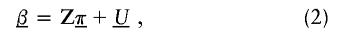
Z is a second-stage design matrix containing information about the relations among markers,  is a column vector of coefficients corresponding to the effects on disease of the marker-specific relations defined in Z,
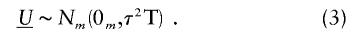
  are random effects reflecting the residual log odds ratio after adjustment for marker level risk factors and/or marker level relations defined in Z, 0_m_ is an m × 1 vector of zeros, and τ2T is an m × m covariance matrix.
Z incorporates into a second stage the chromosomal structure of the genetic markers, whereby the estimate of each β_m_ “borrows” information from the other estimates. For example, recent work shows the potential for markers to cluster into regions of high inter-marker linkage disequilibrium or haplotype blocks, separated by localized hot spots of recombination (Daly et al. 2001; Goldstein 2001; Jeffreys et al. 2001; Johnson et al. 2001; Reich et al. 2001; Gabriel et al. 2002; Patil et al. 2001). For such genetic structure, the Z matrix could be composed of indicator variables distinguishing which markers are in a particular haplotype block or cluster. Those within the same block would thus borrow information from one another to improve estimation. Moreover, the estimated  reflect the effect of each haplotype block on disease.
The residual variability for the measures of LD may be incorporated in a second-stage model through the specification of the covariance matrix, τ2T, for the random effects,  . This is essentially a smoothing parameter, where τ2 controls the overall level of smoothing, and the structure of T defines the intricacies of the smoothing. If there is only unstructured variability along the chromosome, T can equal the identity matrix. If we believe that the residual effects have a spatial dependence, as is likely for measures of LD along particular chromosomal segments, we can model the log of the odds ratios with a spatially structured model (Richardson et al. 1992; Pascutto et al. 2000). Here, we can specify T with a distance function, t _ml_=g(d ml,Θ), where d ml is the distance between marker m and marker l, and Θ represents additional parameters that are needed to define the spatial dependence between m and l. For fine-scale mapping, we can use a general exponential decay function of spatial dependence relative to inter-marker distance (Wakefield et al. 2000),
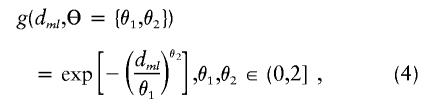
where θ1 and θ2 determine the degree of spatial dependence and the distance, d ml, can reflect marker adjacency, or physical or genetic distance between markers. Here, we prespecified θ1 and θ2. For positive spatial dependence, θ2 is restricted, because θ2>2 results in a covariance matrix with both theoretical and practical difficulties (Diggle et al. 1998). One may also choose to estimate the spatial dependence from the data (Wakefield et al. 2000).
The final structure of T is a function of the distance metric used for d ml and our prior belief in the spatial dependence between the markers. By defining distance as a function of adjacency, we assume that the distance between each marker is uniform across the chromosomal region. If more information is available regarding map locations, then more accurate spatial relations may be specified using physical or genetic distance for d ml. Although either distance provides additional resolution, the most appropriate choice is that which best reflects the spatial dependence between the markers. For certain sets of markers, genetic distance may best reflect the spatial dependence due to recombination. Nevertheless, previous work on hierarchical modeling shows that subtle differences in specification of the second-stage model do not necessarily have a large impact on the improvement available with this approach (Witte and Greenland, 1996). To fit the hierarchical model, one can use a two-stage estimation procedure (see appendix A).
Simulation Study
To evaluate the potential gains of a spatially structured HLD model over conventional pairwise LD, we undertake a fundamental simulation study. Specifically, we use a forward-in-time procedure to simulate a chromosomal region with a single causal variant and an expected unimodal pattern of LD. We ignore mutation to evaluate the resulting variation in the measures of LD due only to recombination, allele frequency differences across the markers on the chromosome, differences in attributable fractions for the causal variant, and limited stochastic evolution (i.e., variation resulting from population history). Although a coalescent model may allow for simulations that are more representative of certain human populations, we simulate under optimal conditions for conventional pairwise LD (i.e., expected unimodal pattern and restricted causes of variation) to gauge any potential improvement using HLD.
For each of 1,000 trials, we simulate a population of 20,000 individuals with a disease prevalence of 5% and allow them to mate randomly for 50 generations. We then sample 500 case individuals and 500 control individuals from the resulting population. Fourteen SNPs are initially in complete disequilibrium (i.e., _D_′=1 for all markers) with a simulated disease polymorphism, located halfway between the seventh and eighth SNPs. Recombination is simulated as a Poisson process with the rate determined by the SNP spacing along the chromosome. We simulate scenarios with a range of locations and allele frequencies for the SNPs, various disease allele frequencies, multiple attributable fractions, and genetic relative risks for the disease polymorphism (described in table 1). The specific genetic model for each scenario is defined by the following equations for the disease prevalence

the attributable fraction
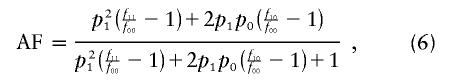
and the relation of the penetrances (Kaplan and Morris 2001)
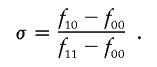
For all the scenarios, we assume that _f_11>_f_10>_f_00 and σ=0.5 (i.e., an additive model).
Table 1.
Results from Simulation Study Comparing Conventional Linkage Disequilibrium with Hierarchical Linkage Disequilibrium (HLD)
| Ratio of HLD to First-Stage LDg | ||||||||||||||
|---|---|---|---|---|---|---|---|---|---|---|---|---|---|---|
| First-Stage LD | τ=.05 | τ=.1 | τ=.15 | |||||||||||
| Scenario | MarkerAlleleFrequencies | MarkerSpacing (cM) | _p_1a | AFb | GRRc | GRRd | Neare | MSEf | Near | MSE | Near | MSE | Near | MSE |
| 1 | Constant (.5) | Constant (.5) | .3 | .6 | 3.5 | 6.0 | 91.1 | .11 | 1.06 | .36 | 1.04 | .51 | 1.03 | .68 |
| 2 | Constant (.5) | Constant (.5) | .3 | .3 | 1.7 | 2.4 | 60.5 | 2.00 | 1.14 | .69 | 1.12 | .77 | 1.08 | .85 |
| 3 | Constant (.5) | Constant (.5) | .3 | .1 | 1.2 | 1.4 | 28.0 | 9.30 | 1.01 | 1.00 | 1.01 | .98 | 1.01 | .98 |
| 4 | Constant (.1) | Constant (.5) | .3 | .6 | 3.5 | 6.0 | 71.8 | .89 | 1.20 | .32 | 1.19 | .35 | 1.18 | .39 |
| 5 | Constant (.1) | Constant (.5) | .3 | .3 | 1.7 | 2.4 | 45.9 | 4.36 | 1.29 | .66 | 1.30 | .66 | 1.24 | .71 |
| 6 | Constant (.1) | Constant (.5) | .3 | .1 | 1.2 | 1.4 | 23.4 | 9.62 | 1.08 | 1.02 | 1.09 | 1.04 | 1.06 | 1.05 |
| 7 | Constant (.5) | Random (.3–.8) | .3 | .6 | 3.5 | 6.0 | 91.9 | .10 | 1.05 | .35 | 1.05 | .37 | 1.03 | .59 |
| 8 | Constant (.5) | Random (.3–.8) | .3 | .3 | 1.7 | 2.4 | 62.4 | 2.05 | 1.15 | .52 | 1.12 | .60 | 1.08 | .73 |
| 9 | Constant (.5) | Random (.3–.8) | .3 | .1 | 1.2 | 1.4 | 28.3 | 8.52 | 1.06 | 1.05 | 1.08 | 1.03 | 1.05 | 1.03 |
| 10 | Random (.1–.9) | Constant (.5) | .3 | .6 | 3.5 | 6.0 | 71.0 | .64 | 1.03 | .66 | 1.02 | .70 | 1.03 | .72 |
| 11 | Random (.1–.9) | Constant (.5) | .3 | .3 | 1.7 | 2.4 | 56.0 | 2.46 | 1.03 | .77 | 1.07 | .71 | 1.09 | .77 |
| 12 | Random (.1–.9) | Constant (.5) | .3 | .1 | 1.2 | 1.4 | 23.8 | 9.89 | 1.18 | .96 | 1.16 | .96 | 1.14 | .96 |
| 13 | Random (.1–.9) | Random (.3–.8) | .3 | .6 | 3.5 | 6.0 | 72.3 | .64 | 1.02 | .82 | 1.02 | .78 | 1.03 | .82 |
| 14 | Random (.1–.9) | Random (.3–.8) | .3 | .3 | 1.7 | 2.4 | 56.2 | 2.65 | 1.06 | .77 | 1.08 | .79 | 1.06 | .82 |
| 15 | Random (.1–.9) | Random (.3–.8) | .3 | .1 | 1.2 | 1.4 | 27.2 | 9.13 | .98 | 1.02 | 1.03 | 1.01 | 1.00 | 1.00 |
| 16 | Constant (.5) | Constant (.5) | .1 | .6 | 8.5 | 16.0 | 88.2 | .19 | 1.09 | .19 | 1.09 | .26 | 1.06 | .40 |
| 17 | Constant (.5) | Constant (.5) | .1 | .3 | 3.1 | 5.3 | 62.1 | 1.84 | 1.18 | .48 | 1.13 | .63 | 1.10 | .74 |
| 18 | Constant (.5) | Constant (.5) | .1 | .1 | 1.6 | 2.1 | 28.9 | 8.54 | 1.08 | .98 | 1.06 | .97 | 1.07 | 1.01 |
| 19 | Constant (.5) | Constant (.5) | .5 | .6 | 2.5 | 4.0 | 98.7 | .01 | 1.00 | .69 | 1.01 | .54 | 1.01 | .46 |
| 20 | Constant (.5) | Constant (.5) | .5 | .3 | 1.4 | 1.9 | 77.2 | 1.50 | 1.02 | .90 | 1.03 | .87 | 1.02 | .94 |
| 21 | Constant (.5) | Constant (.5) | .5 | .1 | 1.1 | 1.2 | 31.3 | 9.44 | 1.04 | .98 | 1.07 | .99 | 1.03 | .98 |
To analyze the resulting case-control data, we use a first-stage logistic regression with a log-additive coding (δ=0.5) for the genotypes at each SNP. The second-stage model is spatially structured, with the dependence determined by an exponential decay function (eq. [4], θ1=1,000, θ2=1) to define the second-stage correlation matrix, T, and a 14 × 1 vector of ones for the second-stage design matrix, Z. This should smooth the first-stage estimates towards a global mean—the extent of smoothing for each marker defined by the inverse-variance weight (A2) and the estimates of the surrounding markers. We fit the model with three prespecified values for τ (0.5, 0.1, 0.15), to test the sensitivity of the posterior estimates.
The performance of these models is assessed with the following two measures (Devlin and Risch 1995): (1) the number of times in 1,000 trials that the marker with the largest measure of LD is next to the disease-causing polymorphism (Near); and (2) the mean squared error using the distance from the disease locus to the marker with the highest measure of LD, given in number of markers (MSE). The first reflects localization of the disease-causing SNP, and the second refinement of the LD pattern.
The results from the simulation study are presented in table 1. For comparison, we give the observed values for the conventional first-stage LD, and the ratio of the HLD results to these values (i.e., calculated by dividing the performance measure for HLD by the corresponding measure obtained from the conventional first-stage analysis). Hence, a ratio of 1.0 indicates that the conventional and HLD approaches give identical results; departures from 1.0 show the improvement of one approach over the other. In particular, ratios above 1.0 for Near and below 1.0 for MSE indicate improvement of HLD over the conventional one-stage analysis.
In 111 of 126 measurements, HLD did better than LD, with four measures indicating equivalent performance. Across all scenarios, the total average ratio for Near shows that there is an 8% increase in the performance of HLD over LD in localizing the disease-causing gene (table 2). Additionally, HLD substantially reduces MSE (a 25% reduction, on average), indicating a considerable refinement in the LD pattern. The trend of the average ratio across each attributable fraction (AF) shows a maximum improvement for locating the disease locus when the AF is modest, _AF_=0.3 (an 11% increase, on average, for Near). This improvement is smaller for more extreme values (i.e., _AF_=0.1 and _AF_=0.6), with an average of a 6% increase in performance. For pattern refinement, as indicated by MSE, the maximum improvement from using HLD occurs for high AF (a 48% reduction on average for MSE). This improvement decreases as the AF decreases. Furthermore, the average ratio within each AF shows that HLD improves upon conventional LD across all the three prespecified values for τ, with a slight trend of increased relative performance as τ decreases.
Table 2.
Results from Simulation Study Comparing Conventional Linkage Disequilibrium with Hierarchical Linkage Disequilibrium (HLD)
| Ratio of HLD to First-Stage LD | ||||||
|---|---|---|---|---|---|---|
| τ=.05 | τ=.1 | τ=.15 | ||||
| AverageValuefor | Near | MSE | Near | MSE | Near | MSE |
| _AF_=0.6 | 1.06 | .48 | 1.06 | .50 | 1.05 | .58 |
| _AF_=0.3 | 1.12 | .68 | 1.12 | .72 | 1.09 | .79 |
| _AF_=0.1 | 1.06 | 1.00 | 1.07 | 1.00 | 1.05 | 1.00 |
| Overall | 1.08 | .72 | 1.08 | .74 | 1.07 | .79 |
For the simple situations when the marker allele frequencies are moderate and constant, the marker spacing is constant, and the disease allele frequency is modest (scenarios 1–3), HLD demonstrates both an improvement in the localization (Near) and in pattern refinement (MSE). When scenarios 1–3 are used as a standard for comparison, and when the marker allele frequencies are rare but remain constant (scenarios 4–6), the first-stage LD estimates perform poorly. For these scenarios, there is an increase in the relative improvement of HLD to detect the disease locus. Randomization of the marker spacing (scenarios 7–9) has little effect on the performance of the first-stage estimates and the relative increase in performance using HLD. Fluctuations in the pattern of the log odds ratio are greatest when the marker allele frequencies vary along the chromosomal region. This is reflected in the decreased performance of the first-stage LD estimates when the allele frequencies are randomized (scenarios 10–15). While the ability of HLD to improve upon the first-stage estimates is maintained for these situations, its relative improvement over conventional LD is diminished. Finally, when the disease allele frequency is rare (scenarios 16–18), HLD shows greater improvement for localization and pattern refinement. Increasing the disease allele frequency (scenarios 19–21) results in better performance of the first-stage estimates. As conventional LD performance increases, it is more difficult for HLD to demonstrate dramatic improvements. Nevertheless, HLD is still able to enhance conventional estimation and clarify the LD pattern.
Application of HLD
We illustrate HLD with data previously used to examine the pattern of LD and the underlying haplotype structure for a 500-kb region on chromosome 5q31 (Daly et al. 2001). The data consist of 103 “common” SNPs (i.e., with minor allele frequencies >5%). Daly et al. (2001) used a hidden Markov model to determine 11 haplotype blocks (groups of loci with low diversity), presumably separated by local hotspots of recombination. They then used this underlying block information to refine the pattern of LD. We extend this work by using the haplotype blocks in a hierarchical model. This results in the individual pairwise estimates of LD “borrowing” information from all the markers within the same block.
To approximate a conventional population-based case-control study, we select the offspring in each of 129 family trios for analysis. Similar to Daly et al. (2001; see their fig. 1_c_ and 1_d_), we used SNP 61, located at 579 kb, as the disease-causing locus. For our analyses, the frequency of the disease allele at SNP 61 is 30%, resulting in 30% of the sample being defined as cases, and the remaining 70% as controls. Individuals with missing data for SNP 61 were excluded from our application, leaving 105 individuals and 97 noncausal SNPs for the analysis.
Our aim is to examine how the pattern of LD for the 97 noncausal SNPs is refined under different specifications of the hierarchical model and varying levels of information. For all analyses, we choose to examine the log of the odds ratio associated with a single allele increase as our measure of LD and we investigate three second-stage models (denoted here as “A,” “B,” and “C”). Model A is a spatially structured model with the relations in the residual matrix, T, determined by an exponential decay function (5), where θ1=7,000, θ2=1, and d ml equals the distance, in bases, between two markers. The second-stage design matrix, Z, is a 97 × 1 vector of ones. In general, this model will shrink the first-stage estimates toward a global mean for all the markers, using the spatial relations of the surrounding markers to determine the degree of shrinkage for each marker.
Model B is an unstructured hierarchical model with T equal to the identity matrix and the second-stage design matrix, Z, determined by the underlying haplotype block structure defined by Daly et al. (2001) (fig. 1). We assigned four SNPs not classified by Daly et al. (2001) to the block immediately upstream. In model B, the HLD estimates are a weighted average of the first-stage pairwise estimates and the second-stage means for each haplotype block,  . By using an unstructured residual variance, we assume that it is uniform across all markers within the chromosomal region. Model C is a spatially structured model combining the properties of models A and B to incorporate both spatial dependence and block information. The HLD estimates will be weighted toward the second-stage means for each haplotype block with the extent of shrinkage determined by the spatial dependence of each marker along the chromosomal region. To examine the sensitivity of the HLD estimates to τ, all models were performed using three different values for τ (0.2, 0.35, and 0.5).
Figure 1.

Second-stage design matrix using the haplotype blocks and SNP labels from Daly et al. (2001).
Figure 2 presents patterns of LD for the first-stage, second-stage, and hierarchical model estimates. The first-stage log odds ratios yield a peak, at the location of the disease-predisposing locus, more distinct than the measure of D′ used by Daly et al. (2001). Note, however, that the resulting pattern of LD from our analysis using the log of the odds ratio is not directly comparable to the analysis in Daly et al. (2001), which aims to examine the underlying haplotype relations using D′, a measure sensitive mostly to recombination. Although the two highest first-stage estimates of LD are located adjacent to the disease locus at SNP 62 and SNP 63, greater dependence of the log odds ratio on allele frequency results in increased variability in the estimates across the chromosomal region, compared with D′. For example, in the region from 520 to 620 kb, the range of the first-stage estimates of the log odds ratio is large, from 0.54 (SNP 75) to 6.13 (SNP 62). In contrast, for model A with τ=0.35 in figure 2, the range of estimates is much smaller, from 1.82 (SNP 75) to 4.41 (SNP 60). Reducing the variability for all of the estimates refines the overall pattern of LD and clarifies the region with the disease predisposing locus. By defining Z with marker inclusion into haplotype blocks, each estimated second-stage effect,  , is equal to the mean for all markers within the same block. The patterns of these estimates provide additional support for localizing the disease. However, instead of relying solely on the haplotype block estimates, HLD incorporates this information to reduce the variability in the pairwise measures of LD. As demonstrated in figure 2 , model B, we maintain the ability to resolve the disease location that is provided by the HLD pairwise measures, while gaining regional support from the second-stage estimates.
Figure 2.

Linkage disequilibrium patterns for the Daly et al. (2001) data using spatial relations only (model A), haplotype blocks (model B), and both spatial relations and haplotype blocks (model C). Unblackened circles (○) indicate the first-stage estimates of the log odds ratio. Blackened circles (●) indicate the HLD estimates from the corresponding hierarchical model. The solid lines are the second-stage regression coefficients,  . The vertical dashed line identifies the location of the “disease” locus at SNP 61 (579 kb).
The measures of LD in the 100-kb region around the predisposing locus, which correspond to block 7 in Daly et al. (2001) (515 kb to 615 kb), help to elucidate the influence of spatial dependence and genetic structure. Focusing on the models with τ=0.35 in figure 3, the spatially structured model A only slightly reduces the variation in the estimates, but maintains the ability to locate the disease-causing locus. For model B, the heavy weighting of the first-stage estimates toward the second-stage mean for block 7 greatly reduces their variability, but the resolution of the LD peak is substantially diminished. In contrast, model C reduces the variation in LD estimates and maintains the ability to resolve the location of the disease-causing locus. Thus, as we move from treating the markers as independent to incorporating more intermarker relations, our ability to reduce the fluctuations in the pattern of LD and to localize the disease gene increases.
Figure 3.

Shrinkage of conventional linkage disequilibrium estimates by hierarchical modeling. The first-stage estimates of the log odds ratio (LD) and the SEs are paired with the corresponding posterior estimates from the hierarchical model (HLD). For the log odds ratio, the first-stage LD estimates are shrunk toward the second stage global mean for model A, 2.04. The degree of shrinkage reflects the value of τ.
Figure 3 demonstrates the shrinkage of the first-stage log odds ratios toward the second-stage mean, a corresponding reduction of the SEs, and the sensitivity of the results to the choice of τ. Model A with τ=0.2 shows a substantial amount of weighting of the first-stage log odds ratios towards the second-stage global mean, 2.04. In addition, there is a considerable decrease in the SEs associated with the final HLD estimates. In comparison—and as expected—the model with τ=0.5 shows less weighting towards the second-stage mean; the first-stage estimates dominate the HLD estimates obtained from equation (A1). In parallel, there is also less reduction in the SEs.
As noted in the methods section, the amount of shrinkage of the first-stage log odds ratio toward the second-stage mean is a function of the precision of the first-stage estimates. This is illustrated by examining two SNPs (45 and 46) within block 7 (table 3). Although SNPs 45 and 46 have similar first-stage estimates, the SE of the log odds ratio for SNP 45 is much greater, resulting in more shrinkage toward the second-stage mean and thus, different HLD estimates.
Table 3.
Illustrative Results Comparing Conventional Linkage Disequilibrium (LD) to Hierarchical Linkage Disequilibrium (HLD)[Note]
| Log Odds Ratio (SE) | |||
|---|---|---|---|
| SNP | Location(kb) | First-Stage LD | HLD Model Ba |
| 45 | 520 | 2.90 (1.08) | 3.46 (.35)b |
| 46 | 522 | 3.02 (.42) | 3.32 (.27)b |
In addition to this case-control illustration, we use HLD to investigate the association between the 103 SNPs in the 5q31 region and Crohn disease (Rioux et al. 2001). Specifically, with the original 129 family trios, we use a transmission/disequilibrium test (TDT) analysis to obtain first-stage estimates of LD (Spielman and Ewens 1996). We then apply hierarchical model C, using the exponential decay spatial dependence and haplotype block information (fig. 1) in an attempt to refine the pattern of LD. Rioux et al. (2001) determined 11 SNPs that are unique to the risk haplotype (table 4). Although these SNPs contain very similar genetic information in terms of their ratio of transmitted to untransmitted chromosomes and their underlying haplotype, HLD distinguishes the effect of the individual SNPs on Crohn disease, with the incorporation of spatial dependence and block structure. Along the entire 5q31 region, HLD refines the LD pattern (fig. 4). We observe substantial support for an association within an ∼250–350 kb region, as seen in the work of Rioux et al. (2001). Moreover, the HLD analysis implicates two narrow peaks, centered approximately at 435 kb and 620 kb, and provides additional support from the second-stage effect estimates for each haplotype block.
Table 4.
LD Mapping for 5q31 and Crohn Disease
Figure 4.

Linkage disequilibrium patterns for Crohn disease for a 103 SNPs in the 5q31 region. Unblackened circles (○) indicate the first-stage estimates of the odds ratio obtained from a TDT analysis. Blackened circles (●) indicate the HLD estimates from a hierarchical analysis with both spatial relations and haplotype blocks (model C with τ=0.35). The solid lines are the second-stage regression coefficients,  for each haplotype block. For comparison to figure 3 from Rioux et al. (2001), the figure is truncated at an odds ratio of 3.0, thus removing SNP 79 at 617 kb with an odds ratio of 4.5.
Discussion
We demonstrate here how one can use HLD for fine-scale mapping of disease genes. This approach incorporates higher-level information on genetic structure and the spatial relations of markers along a chromosomal region to improve the localization of disease-causing genes. HLD has two primary effects on estimates of LD. First, the inverse variance weighting of the first- and second-stage estimates yield final HLD estimates which are more stable when the data are sparse. Second, “borrowing” information from surrounding markers may reduce the impact that population history and structure have on LD estimation. This results in more stable estimates of LD and increased clarity in the interpretation of LD patterns. Our simulation study indicates that this improvement can be substantial. For modest attributable fractions the resolution of the disease gene location is greatly enhanced, while improved pattern refinement occurs for higher attributable fractions. The flexibility and potential value of HLD is further shown in our applications to the data from Daly et al. (2001) and Rioux et al. (2001), where the incorporation of both spatial relations and genetic structure refines the pattern of LD, provides regional support through haplotype block effect estimates, and increases the precision of the pairwise estimates of LD.
In related work, methods have been developed for incorporating the correlations that exist among neighboring markers across chromosomal regions. Lazzeroni (1998) and Cordell and Elston (1999) apply curve-fitting procedures across the first-stage estimates by integrating marker correlations into the fitting process. If haplotype information is available, these methods may use a bootstrap or multinomial approximation to estimate the first-stage covariance matrix,  . An extension of these approaches could use this estimated correlation matrix in a hierarchical model, in which spatial relations are also included. The final posterior estimates would be a weighted average based upon the estimated sampling variation and the prior spatially structured variance (A2). Another recent approach to LD mapping entails modeling the underlying genetic haplotype structure and genealogies with complex functions of the data’s joint likelihood (McPeek and Strahs 1999; Service et al. 1999; Morris et al. 2000; Liu et al. 2001). Although these methods show promise, they are computationally intensive and rely heavily on the ability to estimate many population genetic parameters.
All of the above approaches can be viewed as hierarchical models (Clayton 2000). For a second-stage distribution, the approaches of Lazzeroni (1998) and Cordell and Elston (1999) focus on incorporating correlations along the chromosome, while the joint likelihood approach attempts to estimate the correlations, among haplotypes, due to population history. Our hierarchical model incorporates both of these aspects: correlations along the chromosome, by applying a spatial structure based on the predicted decay of LD, and relations among haplotypes, by including haplotype block structure in the second-stage design matrix.
With multiple markers in a chromosomal region, one can also undertake a haplotype-level analysis. This approach examines the association of combinations of alleles across several markers with the disease phenotype (Schaid et al. 2002; Zaykin et al. 2002). However, difficulties arise in determining which markers are in the haplotypes, how to estimate these haplotypes within population-based samples (Fallin and Schork 2000), and how to analyze the numerous haplotypes that result when multiple markers are involved (Clayton and Jones 1999; Fallin et al. 2001). When individual markers are grouped, there is the potential for increased power (Bader 2001; Kaplan and Morris 2001; Morris and Kaplan 2002), but these methods only give an estimate of the joint effect for the grouped markers. Thus, refinement of the location of a disease polymorphism along the chromosome within an associated group or haplotype is not possible.
In contrast, incorporating the underlying haplotype structure into a hierarchical model can result in estimates for each marker that are weighted between conventional pairwise measures of LD and haplotype-level associations from haplotype blocks or marker groups. In fact, one often analyzes fine-scale genetic data with a two-step process, first calculating the pairwise measures of LD and then exploring the haplotype effects. HLD offers a way to integrate both approaches—an advantage when only genotype level data is available and haplotypes must be estimated. The estimated haplotypes can then be included in the analysis to refine the pattern of pairwise LD, without relying solely upon estimated effects obtained from the inexact haplotypes.
A key step in HLD is specification of τ. Although prespecifying τ and using a two-stage estimation procedure may underestimate the posterior variance, we are primarily interested in evaluating the pattern of LD that is reflected in the posterior log odds ratio estimates. Uncertainty in τ can be incorporated with Markov chain–Monte Carlo methods for parameter estimation (Gilks et al. 1996). For example, an analysis of chromosome 5q31 data (Daly et al. 2001) using model B and WinBUGS (Spiegelhalter et al. 1999), estimates τ=0.55. However, prespecification and sensitivity analysis using various values of τ allow exploration of the changing pattern of LD with varying influence of the prior information. Such an analysis may give important insight into which markers and regions provide the most reliable and stable estimates for the interpretation of the pattern of LD.
Although our findings demonstrate the promise of HLD, we are limited by building on conventional pairwise estimates and their ability to provide LD in the presence of increased stochastic variability. This may hinder our capacity to localize a disease locus when the attributable fraction is small and the marker allele frequencies vary considerably along a chromosomal region. Another potential limitation is that, although the addition of prior information can dramatically improve estimation, it can bias the final estimates. However, if the information used is fairly accurate, the reduction in the variance for the final estimates will far outweigh this bias, yielding estimates that are more precise in terms of reduced mean-squared errors (Greenland 2000_a_).
The methods presented here offer a flexible approach to incorporate higher-level genetic information within a wide variety of data structures. When information exists on marker location and haplotype structure, it can be used in a HLD approach to improve conventional LD estimates. A generalized linear mixed model (GLMM) allows for extension of the first stage to data from family-based studies (Self et al. 1991; Schaid 1996; Abecasis et al. 2000) and various disease outcomes (George et al. 1999; Li and Fan 2000). Furthermore, although this approach has been presented in the context of fine-scale disease mapping by use of the log odds ratio, stable estimates from HLD may facilitate examination of population dynamics when comparing LD patterns obtained from any pairwise measure of LD. HLD can be implemented in standard statistical software packages (Witte et al. 1998, 2000) and scripts for undertaking this analysis can be downloaded from our Web site.
Acknowledgments
We thank the reviewers and Sander Greenland for helpful suggestions on this paper. This work supported in part by grants from the National Institutes of Health (CA88164 and HL07567).
Appendix: HLD Estimation
HLD estimates may be obtained by combining the first- and second-stages in a semi-Bayes, empirical Bayes, or fully Bayesian approach (Gelman et al. 1995; Greenland 1997). For computational ease and conceptual simplicity, we use a semi-Bayes approach with a two-stage estimation procedure. A semi-Bayes approach may also be viewed as a sensitivity analysis in which the influence of second-stage information is varied in a hierarchical model (Greenland and Poole 1994). In two-stage estimation, a first-stage regression model is fitted by use of conventional logistic regression to obtain the estimates of  ,
,  , and their SEs. Note that a separate first-stage regression is undertaken for each marker, because high colinearity among neighboring markers may lead to difficulties in fitting a first-stage model that includes all markers (Neter et al. 1996). Additionally, because, in fine-scale mapping, the association between each individual marker and disease contributes to the overall pattern of LD, one should not condition on additional markers when obtaining the estimate of effect for each marker.
The second-stage estimated prior means, , and corresponding estimated covariance matrix,
  , can be obtained from a weighted least squares regression,
  , where
  , and
, and  is a diagonal matrix with elements equal to the square of the estimated SEs for
  (Morris 1983). Averaging the first- and second-stage estimates yields HLD estimates
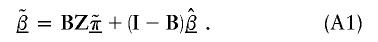
The estimate of the HLD covariance matrix is given by  , where
 and B is the estimated shrinkage matrix
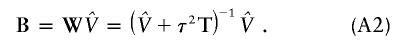
From (A2), if the maximum-likelihood first-stage estimates,  , have large variance,
  , relative to the prior variance, τ2T, then B will also be large. This will result in HLD estimates from (A1) weighted more heavily toward the conditional second-stage mean,
  . Conversely, if the first-stage estimates have small variances, B will be small, resulting in final estimates,
 , close to the first-stage estimates,
  .
.
In semi-Bayes, τ2T is prespecified. If it equals infinity, we see from (A1) and (A2) that all second-stage information is ignored, and the HLD estimate is equal to the first-stage estimates,  . At the other extreme, if τ2 equals zero, the HLD estimates will equal the second-stage conditional means,
  . Intermediate values for τ2 result in shrinkage estimation that is a compromise between the first- and second-stage estimates and reflect the ranges of residual odds ratios for the markers. For example, after accounting for the relations defined in Z, a value of τ=0.354 implies a 95% prior certainty interval of exp(±3.92×0.354)={0.5,2.0} for the residual odds ratio (i.e., a fourfold range) (Greenland 2000_b_).
Electronic-Database Information
Accession numbers and URLs for data presented herein are as follows:
- Authors' Web site, http://darwin.cwru.edu/~witte/software.htm (for script download)
References
- Abecasis GR, Cookson WO, Cardon LR (2000) Pedigree tests of transmission disequilibrium. Eur J Hum Genet 8:545–551 [DOI] [PubMed] [Google Scholar]
- Abecasis GR, Noguchi E, Heinzmann A, Traherne JA, Bhattacharyya S, Leaves NI, Anderson GG, Zhang Y, Lench NJ, Carey A, Cardon LR, Moffatt MF, Cookson WO (2001) Extent and distribution of linkage disequilibrium in three genomic regions. Am J Hum Genet 68:191–197 [DOI] [PMC free article] [PubMed] [Google Scholar]
- Bader JS (2001) The relative power of SNPs and haplotype as genetic markers for association tests. Pharmacogenomics 2: 11–24 [DOI] [PubMed] [Google Scholar]
- Clayton D (2000) Linkage disequilibrium mapping of disease susceptibility genes in human populations. Int Stat Rev 68:23–43 [Google Scholar]
- Clayton D, Jones H (1999) Transmission/disequilibrium tests for extended marker haplotypes. Am J Hum Genet 65:1161–1169 [DOI] [PMC free article] [PubMed] [Google Scholar]
- Collins A, Ennis S, Taillon-Miller P, Kwok PY, Morton NE (2001) Allelic association with SNPs: metrics, populations, and the linkage disequilibrium map. Hum Mutat 17:255-262 [DOI] [PubMed] [Google Scholar]
- Collins FS, Brooks LD, Chakravarti A (1998) A DNA polymorphism discovery resource for research on human genetic variation. Genome Res 8: 1229–1231 [DOI] [PubMed] [Google Scholar]
- Cordell HJ, Elston RC (1999) Fieller's theorem and linkage disequilibrium mapping. Genet Epidemiol 17:237–252 [DOI] [PubMed] [Google Scholar]
- Daly MJ, Rioux JD, Schaffner SF, Hudson TJ, Lander ES (2001) High-resolution haplotype structure in the human genome. Nat Genet 29:229–232 [DOI] [PubMed] [Google Scholar]
- Devlin B, Risch N (1995) A comparison of linkage disequilibrium measures for fine-scale mapping. Genomics 29:311–322 [DOI] [PubMed] [Google Scholar]
- Diggle PJ, Tawn JA, Moyeed RA (1998) Model-based geostatistics. Appl Stat 47:299–350 [Google Scholar]
- Edwards AWF (1963) The measure of association in a 2 × 2 table. J R Stat Soc A 126:109–114 [Google Scholar]
- Fallin D, Cohen A, Essioux L, Chumakov I, Blumenfeld M, Cohen D, Schork NJ (2001) Genetic analysis of case/control data using estimated haplotype frequencies: application to APOE locus variation and Alzheimer's disease. Genome Res 11:143–151 [DOI] [PMC free article] [PubMed] [Google Scholar]
- Fallin D, Schork NJ (2000) Accuracy of haplotype frequency estimation for biallelic loci, via the expectation-maximization algorithm for unphased diploid genotype data. Am J Hum Genet 67:947–959 [DOI] [PMC free article] [PubMed] [Google Scholar]
- Gabriel SB, Schaffner SF, Nguyen H, Moore JM, Roy J, Blumenstiel B, Higgins J, DeFelice M, Lochner A, Faggart M, Liu-Cordero SN, Rotimi C, Adeyemo A, Cooper R, Ward R, Lander ES, Daly MJ, Altshuler D (2002) The structure of haplotype blocks in the human genome. Science 296:2225–2229 [DOI] [PubMed] [Google Scholar]
- Gelman AB, Carlin JS, Stern HS, Rubin DB (1995) Bayesian data analysis. Chapman and Hall, Boca Raton [Google Scholar]
- George V, Tiwari HK, Zhu X, Elston RC (1999) A test of transmission/disequilibrium for quantitative traits in pedigree data, by multiple regression. Am J Hum Genet 65:236–245 [DOI] [PMC free article] [PubMed] [Google Scholar]
- Gilks WR, Richardson S, Spiegelhalter DJ (eds) (1996) Markov Chain Monte Carlo in practice. Chapman and Hall, Boca Raton [Google Scholar]
- Goldstein DB (2001) Islands of linkage disequilibrium. Nat Genet 29:109–111 [DOI] [PubMed] [Google Scholar]
- Greenland S (1993) Methods for epidemiologic analyses of multiple exposures: a review and comparative study of maximum-likelihood, preliminary testing, and empirical-Bayes regression. Stat Med 12:717–736 [DOI] [PubMed] [Google Scholar]
- Greenland S (1997) Second-stage least squares versus penalized quasi-likelihood for fitting hierarchical models in epidemiologic analyses. Stat Med 16:515–526 [DOI] [PubMed] [Google Scholar]
- Greenland S (2000_a_) Principles of multilevel modelling. Int J Epidemiol 29:158–167 [DOI] [PubMed] [Google Scholar]
- Greenland S (2000_b_) When should epidemiologic regressions use random coefficients? Biometrics 56:915–921 [DOI] [PubMed] [Google Scholar]
- Greenland S, Poole C (1994) Empirical-Bayes and semi-Bayes approaches to occupational and environmental hazard surveillance. Arch Environ Health 49:9–16 [DOI] [PubMed] [Google Scholar]
- Greenland S, Schwartzbaum JA, Finkle WD (2000) Problems due to small samples and sparse data in conditional logistic regression analysis. Am J Epidemiol 151:531–539 [DOI] [PubMed] [Google Scholar]
- Guo G, Wang J (2002) The mixed or multilevel model for behavior genetic analysis. Behav Genet 32:37–49 [DOI] [PubMed] [Google Scholar]
- Hedrick PW (1987) Gametic disequilibrium measures: proceed with caution. Genetics 117:331–341 [DOI] [PMC free article] [PubMed] [Google Scholar]
- Jeffreys AJ, Kauppi L, Neumann R (2001) Intensely punctate meiotic recombination in the class II region of the major histocompatibility complex. Nat Genet 29:217–222 [DOI] [PubMed] [Google Scholar]
- Johnson GC, Esposito L, Barratt BJ, Smith AN, Heward J, Di Genova G, Ueda H, Cordell HJ, Eaves IA, Dudbridge F, Twell RC, Payne F, Hughes W, Nutland S, Stevens H, Carr P, Tuomilehto-Wolf E, Tuomilehto J, Gough SC, Clayton DG, Todd JA (2001) Haplotype tagging for the identification of common disease genes. Nat Genet 29:233–237 [DOI] [PubMed] [Google Scholar]
- Kaplan N, Morris R (2001) Issues concerning association studies for fine mapping a susceptibility gene for a complex disease. Genet Epidemiol 20:432–457 [DOI] [PubMed] [Google Scholar]
- Kim LL, Fijal BA, Witte JS (2001) Hierarchical modeling of the relation between sequence variants and a quantitative trait: addressing multiple comparison and population stratification issues. Genet Epidemiol 21:S668–S673 [DOI] [PubMed] [Google Scholar]
- Lazzeroni LC (1998) Linkage disequilibrium and gene mapping: an empirical least-squares approach. Am J Hum Genet 62:159–70 [DOI] [PMC free article] [PubMed] [Google Scholar]
- Lewontin RC (1988) On measures of gametic disequilibrium. Genetics 120:849-852 [DOI] [PMC free article] [PubMed] [Google Scholar]
- Li H, Fan J (2000) A general test of association for complex diseases with variable age of onset. Genet Epidemiol 19:S43–S49 [DOI] [PubMed] [Google Scholar]
- Liu JS, Sabatti C, Teng J, Keats BJ, Risch N (2001) Bayesian analysis of haplotypes for linkage disequilibrium mapping. Genome Res 11:1716–1724 [DOI] [PMC free article] [PubMed] [Google Scholar]
- McPeek MS, Strahs A (1999) Assessment of linkage disequilibrium by the decay of haplotype sharing, with application to fine-scale genetic mapping. Am J Hum Genet 65:858–875 [DOI] [PMC free article] [PubMed] [Google Scholar]
- Morris AP, Whittaker JC, Balding DJ (2000) Bayesian fine-scale mapping of disease loci, by hidden Markov models. Am J Hum Genet 67:155–169 [DOI] [PMC free article] [PubMed] [Google Scholar]
- Morris C (1983) Parametric empirical Bayes inference: theory and applications (with discussion). J Am Stat Assoc 78:47–65 [Google Scholar]
- Morris RW, Kaplan NL (2002) On the advantage of haplotype analysis in the presence of multiple disease susceptibility alleles. Genet Epidemiol 23:221–233 [DOI] [PubMed] [Google Scholar]
- Neter J, Kutner MH, Nachtsheim CJ, Wasserman W (1996) Applied linear statistical models. McGraw-Hill, Boston [Google Scholar]
- Nordborg M, Tavare S (2002) Linkage disequilibrium: what history has to tell us. Trends Genet 18:83–90 [DOI] [PubMed] [Google Scholar]
- Pascutto C, Wakefield JC, Best NG, Richardson S, Bernardinelli L, Staines A, Elliott P (2000) Statistical issues in the analysis of disease mapping data. Stat Med 19:2493–2519 [DOI] [PubMed] [Google Scholar]
- Patil N, Berno AJ, Hinds DA, Barrett WA, Doshi JM, Hacker CR, Kautzer CR, Lee DH, Marjoribanks C, McDonough DP, Nguyen BT, Norris MC, Sheehan JB, Shen N, Stern D, Stokowski RP, Thomas DJ, Trulson MO, Vyas KR, Frazer KA, Fodor SP, Cox DR (2001) Blocks of limited haplotype diversity revealed by high-resolution scanning of human chromosome 21. Science 294:1719–1723 [DOI] [PubMed] [Google Scholar]
- Pritchard JK, Przeworski M (2001) Linkage disequilibrium in humans: models and data. Am J Hum Genet 69:1–14 [DOI] [PMC free article] [PubMed] [Google Scholar]
- Reich DE, Cargill M, Bolk S, Ireland J, Sabeti PC, Richter DJ, Lavery T, Kouyoumjian R. Farhadian SF, Ward R, Lander ES (2001) Linkage disequilibrium in the human genome. Nature 411:199–204 [DOI] [PubMed] [Google Scholar]
- Richardson S, Guihenneuc C, Lasserre V (1992) Spatial linear models with autocorrelated error structure. Statistician 41:539–557 [Google Scholar]
- Rioux JD, Daly MJ, Silverberg MS, Lindblad K, Steinhart H, Cohen Z, Delmonte T, et al (2001) Genetic variation in the 5q31 cytokine gene cluster confers susceptibility to Crohn disease. Nat Genet 29:223–228 [DOI] [PubMed] [Google Scholar]
- Risch NJ (2000) Searching for genetic determinants in the new millennium. Nature 405:847–856 [DOI] [PubMed] [Google Scholar]
- Sasieni PD (1997) From genotypes to genes: doubling the sample size. Biometrics 53:1253–1261 [PubMed] [Google Scholar]
- Schaid DJ (1996) General score tests for associations of genetic markers with disease using cases and their parents. Genet Epidemiol 13:423–449 [DOI] [PubMed] [Google Scholar]
- Schaid DJ, McDonnell SK, Wang L, Cunningham JM, Thibodeau SN (2002) Caution on pedigree haplotype inference with software that assumes linkage equilibrium. Am J Hum Genet 71:992–995 [DOI] [PMC free article] [PubMed] [Google Scholar]
- Self SG, Longton G, Kopecky KJ, Liang KY (1991) On estimating HLA/disease association with application to a study of aplastic anemia. Biometrics 47:53–61 [PubMed] [Google Scholar]
- Service SK, Lang DW, Freimer NB, Sandkuijl LA (1999) Linkage-disequilibrium mapping of disease genes by reconstruction of ancestral haplotypes in founder populations. Am J Hum Genet 64:1728–1738 [DOI] [PMC free article] [PubMed] [Google Scholar]
- Sillanpaa MJ, Kilpikari R, Ripatti S, Onkamo P, Uimari P (2001) Bayesian association mapping for quantitative traits in a mixture of two populations. Genet Epidemiol 21: S692–S699 [DOI] [PubMed] [Google Scholar]
- Spiegelhalter DJ, Thomas A, Best NG (1999) WinBUGS version 1.2 user manual. MRC Biostatistics Unit, Cambridge, United Kingdom [Google Scholar]
- Spielman RS, Ewens WJ (1996) The TDT and other family-based tests for linkage disequilibrium and association. Am J Hum Genet 59:983–989 [PMC free article] [PubMed] [Google Scholar]
- Thomas DC, Morrison JL, Clayton DG (2001) Bayes estimates of haplotype effects. Genet Epidemiol 21:S712–S717 [DOI] [PubMed] [Google Scholar]
- Wakefield JC, Best NG, Waller LA (2000) Bayesian approaches to disease mapping. In: Elliot P, Wakefield JC, Best NG, Briggs DJ (eds) Spatial epidemiology: methods and applications. Oxford University Press, Oxford, pp 104–127 [Google Scholar]
- Witte JS (1997) Genetic analysis with hierarchical models. Genet Epidemiol 14:1137–1142 [DOI] [PubMed] [Google Scholar]
- Witte JS, Greenland S (1996) Simulation study of hierarchical regression. Stat Med 15:1161–1170 [DOI] [PubMed] [Google Scholar]
- Witte JS, Greenland S, Kim LL (1998) Software for hierarchical modeling of epidemiologic data. Epidemiology 9:563–566 [PubMed] [Google Scholar]
- Witte JS, Greenland S, Kim LL, Arab L (2000) Multilevel modeling in epidemiology with GLIMMIX. Epidemiology 11:684–688 [DOI] [PubMed] [Google Scholar]
- Zaykin DV, Westfall PH, Young SS, Karnoub MA, Wagner MJ, Ehm MG (2002) Testing association of statistically inferred haplotypes with discrete and continuous traits in samples of unrelated individuals. Hum Hered 53:79–91 [DOI] [PubMed] [Google Scholar]