Membrane Potential and Firing Rate in Cat Primary Visual Cortex (original) (raw)
Abstract
We have investigated the relationship between membrane potential and firing rate in cat visual cortex and found that the spike threshold contributes substantially to the sharpness of orientation tuning. The half-width at half-height of the tuning of the spike responses was 23 ± 8°, compared with 38 ± 15° for the membrane potential responses. Direction selectivity was also greater in spike responses (direction index, 0.61 ± 0.35) than in membrane potential responses (0.28 ± 0.21).
Threshold also increased the distinction between simple and complex cells, which is commonly based on the linearity of the spike responses to drifting sinusoidal gratings. In many simple cells, such stimuli evoked substantial elevations in the mean potential, which are nonlinear. Being subthreshold, these elevations would be hard to detect in the firing rate responses. Moreover, just as simple cells displayed various degrees of nonlinearity, complex cells displayed various degrees of linearity.
We fitted the firing rates with a classic rectification model in which firing rate is zero at potentials below a threshold and grows linearly with the potential above threshold. When the model was applied to a low-pass-filtered version of the membrane potential (with spikes removed), the estimated values of threshold (−54.4 ± 1.4 mV) and linear gain (7.2 ± 0.6 spikes · sec−1 · mV−1) were similar across the population. The predicted firing rates matched the observed firing rates well and accounted for the sharpening of orientation tuning of the spike responses relative to that of the membrane potential.
As it was for stimulus orientation, threshold was also independent of stimulus contrast. The rectification model accounted for the dependence of spike responses on contrast and, because of a stimulus-induced tonic hyperpolarization, for the response adaptation induced by prolonged stimulation. Because gain and threshold are unaffected by visual stimulation and by adaptation, we suggest that they are constant under all conditions.
Keywords: threshold, summation, iceberg, tuning, linearity, orientation, contrast, adaptation, simple cells, complex cells
A mechanism that contributes to the remarkable selectivity of cells in the visual cortex is the action potential threshold. Because neurons in the visual cortex are mostly quiet in the absence of visual stimulation, their average membrane potential at rest must lie somewhat below firing threshold. In principle, therefore, the tuning of the firing responses of visual cortical neurons could represent the tip of an iceberg: just as icebergs are wider below the surface of the water than above it, the tuning of the synaptic inputs to a cell could be broader below threshold than above it. In the domain of orientation selectivity, a comparison of tuning curves measured from the membrane potential (Nelson et al., 1994; Pei et al., 1994; Volgushev et al., 1995, 1996;Ferster et al., 1996; Chung and Ferster, 1998) and from the firing rate (Campbell et al., 1968; Rose and Blakemore, 1974a; Gizzi et al., 1990) suggests that threshold does contribute to the sharpness of tuning. Is this contribution substantial? This question is relevant to the intense debate surrounding the mechanism of orientation selectivity (Reid and Alonso, 1996; Vidyasagar et al., 1996; Sompolinsky and Shapley, 1997): if the sharpening provided by the threshold were prominent, then cells would not need to receive synaptic inputs that are sharply tuned.
Another major theme in the current research on the primary visual cortex centers on simple cells and regards the degree to which the responses of these cells are linear. Linearity was implicit in the original descriptions of simple cells (Hubel and Wiesel, 1962) and was investigated by Movshon et al. (1978a) and by a multitude of subsequent studies (for review, see Carandini et al., 1999). Most of these measurements were performed on the spike responses and were thus limited by the intrinsic nonlinearity of threshold. Intracellular measurements of membrane potential are not subject to this limit but have so far yielded mixed results. Jagadeesh et al. (1993, 1997) argued in favor of the linear model, but Volgushev et al. (1996) found indirect evidence for nonlinearity, and recent measurements of the mean potential responses to gratings (Carandini and Ferster, 1997) suggest that simple cells can be quite nonlinear. Overall, a number of questions remain open, including (1) the degree to which simple cells are nonlinear, (2) the effects of this nonlinearity on their tuning for orientation, and (3) the degree to which complex cells and simple cells differ (and can be distinguished by) their linearity.
In the experiments presented in this paper, we have examined the relationship between membrane potential and firing rate in neurons of the cat visual cortex. We have found that the iceberg effect does contribute significantly to orientation and direction selectivity: the orientation tuning of cortical cells as measured from their action potentials is considerably sharper than the orientation tuning measured directly from the membrane potential.
We have also investigated the linearity of the membrane potential responses and found that threshold also increased the distinction between simple and complex cells. This distinction is commonly based on the linearity of the spike responses to drifting sinusoidal gratings. In many simple cells, such stimuli evoked substantial elevations in the mean potential, which are nonlinear. Being subthreshold, these elevations would be hard to detect in the firing rate responses. Moreover, just as simple cells displayed various degrees of nonlinearity, complex cells displayed various degrees of linearity.
A final issue that we have addressed concerns the relationship between membrane potential and firing rate. We have tested what is perhaps the simplest model for this relationship: the _rectification_model (Granit et al., 1963). This model has been used explicitly or implicitly in much of the literature on the response of visual cortical neurons (Movshon et al., 1978a; Ahmed et al., 1998; Carandini et al., 1999) and postulates that the firing rate is zero below the spike threshold and grows linearly above threshold. We found that the relationship between membrane potential and firing rate is well described by the rectification model. The model cannot of course predict the timing of individual spikes but accurately predicts the slower variations in firing rate in response to visual stimuli.
A preliminary version of the results has been presented in abstract form (Carandini and Ferster, 1998).
MATERIALS AND METHODS
Details of most procedures have been described previously (Ferster and Jagadeesh, 1992; Carandini and Ferster, 1997; Jagadeesh et al., 1997). For those procedures, we give only a summary description here.
Experimental preparation. Young adult cats were anesthetized with intravenous sodium thiopental and placed in a stereotaxic headholder. Paralytic agents (gallamine or pancuronium) were administered to minimize motion of the eyes, and the animals were artificially respirated. Phenylephrine hydrochloride and atropine sulfate were applied to the eyes to retract the nictitating membranes, dilate the pupils, and paralyze accommodation. Contact lenses with artificial pupils (4-mm-diameter) were inserted.
Visual stimulation. Visual stimuli consisted of monocularly presented drifting sine-wave gratings displayed on a Tektronix (Wilsonville, OR) 608 oscilloscope screen using a Picasso stimulus generator (Innisfree, Cambridge, MA). The peak contrast used was 64%, and the mean luminance (kept constant throughout the experiments) was 20 cd/m2. Optimal spatial frequency was determined from computer-generated spatial frequency tuning curves. Grating size, position, and temporal frequency were adjusted to be optimal, usually by hand.
To generate orientation tuning curves, stimuli of 12 different orientations (0–330°) were presented in random order, 4 sec for each orientation. The contrast of the gratings was usually 47%, and the block of stimuli included an additional 4 sec blank screen presentation. This block of 13 stimuli was repeated two to five times for each cell, with a different randomized order each time.
To generate contrast–response curves, stimulus blocks consisted of seven optimally oriented stimuli with contrasts logarithmically spaced between 1 and 64%, which were randomly presented. Test stimuli were 4 sec long and were preceded by 4 sec adaptation stimuli (20 sec before the first test stimulus), as previously described (Carandini and Ferster, 1997).
Intracellular recording. Whole-cell patch recordings in the current-clamp mode were obtained from neurons of area 17 of the visual cortex using the technique developed for brain slices by Blanton et al. (1989). Electrodes were filled with a K+-gluconate solution including Ca2+ buffers, pH buffers, and cyclic nucleotides. Junction potentials were measured to be 10 mV. This value was added to the membrane potentials reported in this study. Input resistance ranged typically between 70 and 250 MΩ. Membrane potentials were low-pass-filtered and digitized at 4 kHz, and the timing of spikes was logged with 250 μsec accuracy.
Response measures. To obtain tuning curves for the membrane potential and spike train responses we considered two response measures, the mean and the modulation. The mean response was the average over the 4 sec stimulus presentation, whereas the_modulation_ was the peak-to-peak amplitude of the best-fitting sinusoid at the stimulus frequency (obtained by fast Fourier transform). For this analysis, individual spikes were treated as Dirac δ functions.
Tuning curves. The orientation tuning of the responses was fitted with a descriptive function. This function is the sum of two Gaussians and is defined on the circle. The two Gaussians are forced to peak 180° apart and to have the same width ς:
| f(O)=R0+Rpe−〈O−Op〉2/(2ς2)+Rne−〈O−Op+180〉2/(2ς2). | Equation 1 |
|---|
In the above expression, O is the stimulus orientation (between 0 and 360°), and the angle brackets indicate angular values expressed between −180 and 180°. The function has five parameters: the preferred orientation,_O_p; the tuning width, ς; the base response, _R_0; and the increment in response at the preferred and null orientations,_R_p and_R_n, which correspond to the heights of the two Gaussians. This function assigns the same tuning width (but not necessarily the same amplitude) to the responses to opposite directions of motion. Consistent with previous results on the tuning of the firing rate responses (Campbell et al., 1968), we found that this constraint was appropriate in all of our data sets.
To allow us to report a single preferred orientation and tuning width for each signal, membrane potential and firing rate, the mean and the modulation for each signal were fitted together. In particular, although the base response and the heights of the two Gaussians were allowed to differ for mean and modulation, an additional constraint was applied such that the fits to these measures had the same preferred orientation, _O_p, and tuning width,ς. This constraint did not noticeably worsen the fits and would not affect the comparisons between the tunings of the membrane potential responses and the firing rate responses, which were fitted independently from one another.
Measures of response tuning. From the parameters of Equation1, it is easy to obtain some widely used measures of response tuning, namely the direction index and the orientation tuning half-width.
The direction index is a common measure of direction selectivity (Schiller et al., 1976; Orban et al., 1981; Reid et al., 1987; Gizzi et al., 1990). We define this index as do Reid et al. (1987), i.e., as the difference in the responses obtained with stimuli of preferred and opposite directions of motion, divided by the sum of those responses. In terms of the parameters of the model, the direction index is then (P − N)/(_P_+ N), where P =_R_p +_R_0 is the response to the preferred direction, and N = _R_n+ _R_0 is the response to the nonpreferred direction.
The tuning half-width is a common measure of the narrowness of orientation tuning (Campbell et al., 1968; Rose and Blakemore, 1974a; Gizzi et al., 1990). It is defined as the half-width of the tuning curve at half the height of the peak. In terms of the parameters of the model, the tuning half-width is simply given by _ς_multiplied by ln(4)1/2 = 1.18.
Coarse potentials and firing rates. To test the rectification model of firing rate encoding, we obtained coarse membrane potential traces and firing rates. The coarse membrane potential traces, V(t), were obtained as follows. First, we identified the time of occurrence of spikes by searching for maxima in the derivative of the membrane potential. We then identified the starting and ending times of the typical spike for each cell, including afterhyperpolarizations. Spikes typically began at_t_0 = − 1 msec (i.e., 1 msec before the peak in rising potential), and ended at_t_1 = 5 msec (mean duration_t_1 −_t_0 was 6.5 msec, ranging from 2.0 to 12.2 msec). To remove the spikes from the traces, we replaced each [_t_0,t_1] epoch with a line joining_V(t_0) to_V(_t_1). This replacement left two small scars, i.e., abrupt changes in the slope of the membrane potential traces at _t_0 and_t_1. Subsequent low-pass filtering of the traces with cutoff frequency of 24 Hz made these transitions invisible. To obtain the firing rate traces,R(t), we simply low-pass filtered the spike trains with the same cutoff frequency used with the membrane potential responses. This frequency, 24 Hz, is low enough that the information about the timing of the individual spikes is mostly lost. We then rectified the resulting firing rates to remove the negative ripples introduced by low-pass filtering.
RESULTS
We recorded intracellularly from 41 cells in the cat primary visual cortex and measured their orientation tuning with drifting sinusoidal gratings. Twenty-nine of these cells responded with at least one spike/sec to stimuli of the preferred orientation. Twenty-eight of these 29 cells had a clear preference for orientation and are the object of this study.
The mean resting potential of the cells was −63 ± 10 mV (mean ± SD; n = 28). The mean spike threshold was −49 ± 7 mV. The spike height was often small compared with values commonly observed in vitro, being on average only 21 ± 15 mV. This small value resulted from the large time constant of the electrodes, which acted as a low-pass filter. Indeed, the spike height was negatively correlated with the spike width. The latter, measured at half-height, was on average 1.6 ± 0.9 msec, but for spikes >40 mV it was always <1 msec. The low-pass filter did not, however, have a significant effect on visually evoked synaptic potentials, because these mostly contain substantially lower frequencies than spikes.
Membrane potential responses to different orientations
From extracellular recordings, it is known that in response to drifting gratings simple and complex cells exhibit rather different spike trains: those of simple cells are strongly modulated at the stimulus frequency, whereas those of complex cells consist principally of an elevation in the mean firing rate (Movshon et al., 1978c; Skottun et al., 1991). The basis for this difference in response is often apparent when the measurements are performed intracellularly. This is illustrated in Figure 1, where the responses evoked by optimally oriented gratings drifting in two different directions are shown for two typical cells, one simple and one complex.
Fig. 1.

Membrane potential responses of two cells to stimuli of preferred orientation drifting in the preferred direction (left) and in the nonpreferred (opposite) direction (right). A, Responses of a simple cell (cell 61). The grating stimulus drifted at 4 Hz. Each bar of the grating elicited a strong modulation in the membrane potential response. B, Responses of a complex cell (cell 24). The grating stimulus drifted at 2 Hz. The responses it elicited contained only a mild component at the stimulus frequency. The dotted horizontal lines indicate the resting potential.
The membrane potential of the simple cell (Fig. 1A) was strongly modulated at the temporal frequency of the stimulus (4 Hz). This modulation was stronger for the stimulus drifting in the preferred direction (left) than in the opposite direction (right). In this cell as well as in all other simple cells in our sample, the modulation in membrane potential was seldom symmetrical around the resting potential of the cell: the membrane potential spent more time above rest than below it. Thus, together with a strong modulation, the membrane potential responses of simple cells exhibited a noticeable increase in their mean.
By contrast, the membrane potential response of the complex cell (Fig.1B) consisted mainly of an elevation in the mean. This elevation was accompanied by a gradual hyperpolarization and reduction in spike frequency during the course of the stimulus presentation, which is most likely a consequence of pattern adaptation (Carandini and Ferster, 1997). In addition, the membrane potential of the complex cell exhibited a weak modulation at the stimulus frequency (2 Hz), which is most visible in the response to the nonpreferred direction. Membrane potential modulations of this sort were not a rare sight in complex cells but were in general substantially smaller than the mean increase in membrane potential. Moreover, although the membrane potential response of many complex cells exhibited strong temporal variations, these temporal variations were often not synchronized with the stimulus, taking the form of seemingly random depolarizing events of 50–500 msec duration (Ferster and Carandini, 1996).
The effects of changing stimulus orientation on the responses of the simple cell are illustrated in Figure 2. Here the responses were averaged over each stimulus cycle, so each trace represents the average response of the cell to the passage of one bar of the grating over the receptive field. The firing rate responses (Fig. 2A) are typical of many simple cells: the cell is strongly tuned for orientation, gives no response to stimuli of nonpreferred orientations, and displays a marked preference for one direction of motion (270°) over the opposite (90°).
Fig. 2.

Cycle averages and spike histograms, as a function of stimulus orientation, for the simple cell in Figure1A. The first column refers to a blank stimulus, and the subsequent columns refer to 12 stimulus orientations, spanning the range between 0 and 360° in 30° steps. Responses are averaged over one stimulus cycle (0.25 sec).A, Firing rate. B, Membrane potential. Cell 61.
The strength of the tuning of the firing rate responses is only partly inherited from the underlying membrane potential responses (Fig.2B) and appears to receive a substantial contribution from the spike threshold. In particular, the tuning of the membrane potential responses appears to be broader than that of the firing rate responses in at least three ways. First, although stimuli at orientations flanking the preferred orientation did modulate the membrane potential and increase the mean membrane potential, they did not elicit firing. Second, the mean membrane potential at all orientations was more positive than in the absence of visual stimulation, an effect that is not visible in the firing rate responses (which were zero in both cases). Third, at the preferred orientation the difference between the firing rate response in the two opposite directions of motion (90 and 270°) was far greater than the differences between the corresponding membrane potential responses.
These same observations can be made for the complex cell shown in Figure 1 (Fig. 3). As in the simple cell, stimuli at all orientations evoked a depolarization relative to rest. Moreover, visual stimuli at orientations surrounding the preferred orientation (30 and 210°) increased the mean membrane potential of the cell but did not elicit substantial firing responses, creating a substantial difference in the orientation tuning width measured from the two types of responses. Finally, the two opposite directions of motion at the preferred orientation (60 and 240°) elicited firing rate responses that were far more dissimilar than the corresponding membrane potential responses.
Fig. 3.

Cycle averages and spike histograms, as a function of stimulus orientation, for the complex cell in Figure1B. Format as in Figure 2. Responses are averaged over one stimulus cycle (0.5 sec). Cell 24.
Orientation selectivity of firing rate and membrane potential responses
To quantify the responses (membrane potential or firing rate) to drifting gratings, we used two measures: mean and modulation. The first is simply the average response measured over the stimulus duration. The second is the peak-to-peak amplitude of the sinusoid at the grating frequency that best fits the response (i.e., two times the amplitude of the first harmonic of the response). If the response were a perfect sinusoid, its modulation would be its peak-to-peak amplitude.
The orientation tuning of the mean and modulation of both the membrane potential and the firing rate responses of the simple cell is illustrated in Figure 4. The modulation component was large and well tuned both in the firing rate (Fig.4B) and in the membrane potential (Fig.4D). The mean component was much smaller but similarly tuned.
Fig. 4.

Orientation tuning of the simple cell in Figures1A and 2. Top, Firing rate.Bottom, Membrane potential. Left, Mean responses. Right, Response modulation.Gray areas indicate confidence intervals for the responses to a blank stimulus. Their width and the length of the error bars on the data points are twice the SE of the measurements. In the_top panels_ the confidence intervals are infinitesimal: the response to the blank was always 0 spikes/sec. The thin curves indicate the fits of a descriptive tuning curve (Eq. 1). The thick lines in the _top panels_indicate the predictions of the rectification model of firing rate, obtained from the membrane potential responses. Cell 61.
For the firing rate, that the mean (Fig. 4A) was tuned similarly to the modulation (Fig. 4B) is simply a consequence of the lack of firing rate responses at rest. Because the resting firing rate was zero, the effect on the mean of an increase in rate in one phase of the responses could not be compensated by a decrease at another phase. For the membrane potential, by contrast, there is no corresponding constraint. Indeed, the lower limit for the membrane potential (the reversal potential of potassium ions) was well below the resting potential of the cells. The similarity in tuning between the mean (Fig. 4C) and the modulation component (Fig. 4D) is caused by the tendency pointed out in the description of Figure 1: the modulation in the membrane potential was larger above the resting potential than below it.
A comparison of the orientation tuning curves for firing rate and membrane potential in Figure 4 confirms that the firing rate responses are more sharply tuned than the membrane potential responses. For example, stimuli flanking the preferred orientation (240 and 300°) gave membrane potential responses that were ∼20% as large as the response at the preferred orientation (270°). Yet the firing rate responses to these stimuli were zero, indicating that the tuning width of the firing rate was smaller than the spacing between orientations (30°). In addition to the width of the tuning, the difference in tuning between membrane potential responses and firing rate responses applies most notably to the relative sizes of the responses to the two opposite directions of motion, 90 and 270°. Although the membrane potential responses to a grating drifting in the 270° direction are only marginally larger than those to a grating drifting in the opposite direction, the difference in firing rate responses in the two conditions is substantial.
A similar analysis in terms of mean and modulation can be performed for the complex cell of Figures 1B and 3. The results of such an analysis are illustrated in Figure5. Consistent with the observations made on the traces, the mean component (Fig. 5C) of the membrane potential response is substantially larger than the modulation component (Fig. 5D). Similarly, the mean component (Fig.5A) of the firing rate response is larger than the modulated component (Fig. 5B). In a complex cell, then, the stimulus tuning is mostly expressed in the left panels, which report the response means.
Fig. 5.

Orientation tuning of the complex cell of Figures1B and 3. Format as in Figure 4. Cell 24.
To compare the tuning of the different response measures, mean and modulation of firing rate and membrane potential, we fitted the responses with the descriptive function in Equation 1 and obtained estimates of the direction index and tuning half-width (see Materials and Methods). Even in the face of the restrictions that we imposed to limit the number of free parameters, the fits were generally good. They are illustrated by the thin curves in Figures 4 and 5 and in many subsequent figures.
The values for the direction index confirm that for the cells in Figures 4 and 5, the encoding of subthreshold events into firing rates substantially increased the selectivity for direction of motion. Indeed, for the simple cell in Figure 4 the direction index was 0.25 for the potential modulation (Fig. 4D) and 0.79 for the modulation of the firing rate (Fig. 4B). For the complex cell in Figure 5 the direction index was only 0.09 for the mean membrane potential (Fig. 5C) and 0.82 for the mean firing rate (Fig. 5A).
On the other hand, the values for the tuning half-width of these two cells do not suggest a substantial difference between firing rate and membrane potential in terms of orientation selectivity. Indeed, for the cell in Figure 4 the tuning half-width was 18° for the firing rate and 21° for the membrane potential, and for the cell in Figure 5 the tuning half-width was similarly narrow in the two signals (17°).
Before concluding that in these cells the encoding of membrane potential into firing rates did not sharpen the tuning, however, one should consider that half-widths of 17–18° are the lowest that can be measured from our data. This limit arises from the 30° spacing of our stimuli on the orientation axis. Because in these two cells the firing rate responses were zero at all orientations except the preferred, it is likely that the true tuning half-width for the firing rate was actually <17°. For the membrane potential, on the other hand, the presence of data points on the slopes of the tuning curves (Figs. 4D, 5C) indicates that the data would not be fitted by narrower tuning curves.
The difference in tuning sharpness between the membrane potential and the firing rate is most evident in cells that are more broadly tuned, where our sampling limitations do not play a role. This is illustrated in Figure 6, which contains the tuning curves for four additional cells, two complex and two simple. For three of these cells, the orientation tuning of the firing rate responses was significantly sharper than that of the membrane potential responses. These are the first complex cell (Fig. 6A–D, half-widths of 23° for the firing rate and 40° for the membrane potential), the first simple cell (Fig. 6I–L, half-widths of 20° for the firing rate and 39° for the membrane potential), and to some degree the second simple cell (Fig.6_M–P_, half-widths of 28° for the firing rate and 38° for the membrane potential). For the second complex cell (Fig. 6E–H), instead, the tuning half-widths of the firing rate and of the membrane potential were similar (28 and 30°).
Fig. 6.

Orientation tunings of two complex cells and two simple cells. The format of each group of four panels is as in Figure4. A–D, E–G, Complex cells (cells 86 and 28).I–L, M–P, Simple cells (cells 68 and 71). These cells are arranged in order of spike modulation index: 0.88, 0.92, 1.43, and 1.54. The corresponding potential modulation indices are 0.41, 0.37, 0.56, and 1.84.
The iceberg effect and orientation selectivity
The narrower tuning of the firing rate responses with respect to the membrane potential responses is a general property of cat V1 cells. The extent of this phenomenon is illustrated in Figure7A, where we compared the tuning width of the two responses as estimated for each cell in our population. The abscissa marks the tuning half-width for the firing rate responses, and the ordinate marks the tuning half-width for the membrane potential. For the overwhelming majority of cells, the points lie to the left of the identity line, indicating that the firing rate was more sharply tuned than the membrane potential. Indeed, the mean tuning width of the firing rate responses was 23 ± 8°, whereas the mean tuning width for the membrane potential was 38 ± 15°. The median difference in tuning width between firing rate and membrane potential responses was 10°. This difference was <2° in one-fourth of the cells and >25° in another fourth of the cells.
Fig. 7.

Comparison of orientation tuning in the membrane potential responses and in the firing rate responses. A, Orientation tuning width at half-height, obtained from fits such as those in Figure 6. B, Direction index, computed from the sum of the mean and modulation components. Open symbols, Simple cells; filled symbols, complex cells.Lines mark the identity between _abscissa_and ordinate.
The degree to which firing rate is more narrowly tuned than membrane potential is even more striking if one considers that we are most likely overestimating the tuning width of the firing rate. As mentioned above, because we sampled the orientation axis in rather coarse, 30° intervals, we cannot resolve orientation tuning curves with half-widths <17°. For half of the cells, this measurement limit was reached by the tuning of the firing rate responses. The half-width of the tuning of these responses was then conservatively estimated to be 17°, resulting in the vertical streak of points in Figure 7_A_. The true half-width for these firing rate responses, however, would lie somewhere to the left of that streak. In most of those cells the half-width of the membrane potential responses was large, often >30°, and if we knew the true half-width of the firing rate, the difference between the two would be even larger than what appears in the graph.
The methods of recording with the whole-cell patch technique are more invasive than those used by most studies of visual responses in cat V1, which were conducted extracellularly. Consequently, it is possible that the firing rate responses that we observed could be unnaturally sharp. For example, the perfusion of the cell with the electrode solution could have altered the resting potential or the amplitude of synaptic potentials of the cells. Some of these possible changes could have generated an artifactual difference in tuning between the membrane potential and firing rate responses.
This concern is soon dispelled when the tuning width of the firing rate responses in our sample is compared with the results of previous extracellular studies (Fig. 8). This comparison suggests that the tuning widths that we report for the firing rate are, if anything, broader than those reported in the literature. An early study of orientation tuning (Campbell et al., 1968) used square grating stimuli and reported a rather large mean tuning half-width of 25 ± 11° (Fig. 8A). A subsequent study used drifting bar stimuli (Rose and Blakemore, 1974a) and reported substantially lower half-widths (Fig.8B). These half-widths had a mode at ∼10–12° and a long tail, yielding a mean value of 18 ± 10°. Similar results were obtained more recently by Gizzi et al. (1990), who used drifting sinusoidal grating stimuli and found a mean half-width of 21 ± 11° but a clearly smaller mode (Fig. 8C). Our data (Fig.8D) seem to be primarily missing this mode: The mean half-width from our cells was 23 ± 8°, and, as explained above, none of our cells could be assigned a half-width <17°. The impression that in many cells we may be overestimating the tuning width of the firing rate responses is thus reinforced by a comparison with the results of previous studies.
Fig. 8.

Orientation tuning of the firing rate responses as measured in published extracellular studies and in our intracellular recordings. The measure of tuning width in the _abscissa_is the half-width at half-height. A, Replotted fromCampbell et al. (1968), who used drifting square grating stimuli.B, Replotted from Rose and Blakemore (1974a), who used drifting bar stimuli. C, Replotted from Gizzi et al. (1990), who used drifting sinusoidal grating stimuli. D, Our data. In all panels, white indicates simple cells,black indicates complex cells, and _gray_indicates unclassified cells.
The iceberg effect and direction selectivity
In addition to being more sharply tuned than the membrane potential responses for stimulus orientation, the firing rate responses tended to be more selective for stimulus direction. This phenomenon has already been reported for simple cells (Jagadeesh et al., 1993, 1997), and we have pointed it out in the simple cell of Figure 4 as well as in the complex cell of Figure 5. An even more striking example is given by the simple cell in Figure 6I–L. In this cell the membrane potential responses (Fig. 6K,L) were only mildly directional, with the responses to the nonpreferred direction (11°) being approximately half as large as the response the preferred direction (191°). Yet the firing rate responses (Fig.6I,J) were completely directional, with the nonpreferred direction eliciting no spikes at all. The direction index computed from the modulated responses was 1.00 for the firing rate (Fig. 6J) and only 0.34 for the membrane potential (Fig. 6L), confirming the substantial difference in direction selectivity between these two attributes of the visual responses.
Comparably dramatic increases in direction selectivity were observed in a number of cells. This property is summarized for all of our cells in Figure 7B, where the direction index (calculated from the sum of the mean and modulation components) is plotted for the membrane potential versus the firing rate responses. Essentially all the points lie on the right side of the identity line, indicating that in the greatest majority of the cases the direction index was higher when measured from the firing rate than when measured from the membrane potential. In only three cells was the direction index of the firing rate smaller than that of the membrane potential (the tuning of one of these cells is in Fig. 6E–H), but these cells were only mildly direction-selective. The average direction index for spikes in our population was 0.61 ± 0.35, whereas the average index for the membrane potential was only 0.28 ± 0.21. This confirms that threshold substantially accentuates direction selectivity in the same way that it does orientation selectivity.
As with the measurements of tuning width, it is of importance to know whether the sampling bias of our technique led us to record from an unnaturally direction-selective set of cells. Again, this concern is dispelled by a comparison with previously published data obtained extracellularly (Gizzi et al., 1990). Using a slightly different definition of direction index than the one used here (1 −N/P, where P is the response to the preferred direction, and N is the response to the nonpreferred direction), Gizzi et al. (1990) found the firing rate responses to have a direction index >0.5 in 64% of cat V1 cells. The direction index was >0.8 in 40% of the cells. If we use the same measure of selectivity in our sample of tuning curves obtained from the firing rate responses, we find 68% of the cells to have a direction index >0.5 and 50% to have a direction index >0.8. The differences between our population and that of Gizzi et al. (1990) are thus minor. A more thorough comparison of the distributions of the direction indices in the two studies as well as a comparison with the results ofReid et al. (1991) confirm that our small sample does not represent an unnaturally selective group of cells.
Nonlinearity of the responses of simple cells
One of the properties implicit in Hubel and Wiesel's (1962)original descriptions of simple cells is the linearity of spatial summation. For example, the response of a simple cell to two stimuli presented simultaneously was reported to equal the sum of the individual responses to the two stimuli presented individually. Hubel and Wiesel's qualitative measurements of summation were tested quantitatively by Movshon et al. (1978a) and by a number of subsequent studies (many of them reviewed by Carandini et al., 1999). But even the most careful quantitative measurements of linearity when performed extracellularly are limited by the intrinsic nonlinearity of spike threshold. Intracellular measurements of membrane potential are not subject to this intrinsic nonlinearity and are thus ideal for estimating the degree of linearity of simple cells (Jagadeesh et al., 1993; Volgushev et al., 1996; Jagadeesh et al., 1997).
In particular, a sensitive assay for nonlinearity is the mean membrane potential response to a sinusoidal grating stimulus. The mean luminance of the stimulus integrated over the receptive field does not change with time, and the mean luminance integrated over time is the same at every point in the receptive field. Furthermore, these means are identical to the luminance of the screen in the absence of a grating. Therefore, for a cell that is summing the inputs from different parts of its receptive field linearly, the mean membrane potential should be unaffected by the grating stimulus.
This was not the case for the simple cells in our sample. As is apparent in the membrane potential traces of Figures1A and 2, the depolarizing events in the responses are larger than the hyperpolarizing events, so that the mean membrane potential is elevated by stimulation. We have observed this elevation previously for stimuli at the preferred orientation (Carandini and Ferster, 1997), and we now report on its tuning for stimulus orientation. As shown in the orientation tuning curves of the three simple cells considered above (in Figs. 4C,6K,O), the mean membrane potential is tuned for stimulus orientation, and its tuning is similar to that of the membrane potential modulation.
In addition to being tuned for stimulus orientation, the mean membrane potential was in many cells higher than at rest for all stimulus orientations. This effect can be observed in Figure9, which shows the fitted tuning curves of the mean and modulation components in the membrane potential for all our cells. An elevation of the mean potential for all orientations was observed in 14 of 21 simple cells (Fig. 9A). It was also observed in six of seven complex cells (Fig. 9C). A few cells, however, displayed the opposite behavior. These cells (four simple and one complex) exhibited a clear reduction in membrane potential at orientations that are close to orthogonal to the preferred orientation. Finally, in all cells the modulation in membrane potential was close to zero for stimuli orthogonal to the preferred orientation.
Fig. 9.
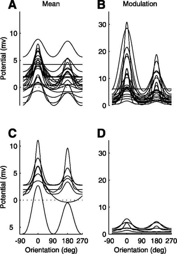
Summary of orientation tuning of the membrane potential. Curves are the fits of the descriptive tuning function (Eq. 1), aligned so that the preferred orientation and direction for the modulated component would be at 0°.A, B, Mean and modulation of membrane potential in 21 simple cells. C, D, Mean and modulation of membrane potential in 7 complex cells.
Having observed a substantial nonlinear component in the responses of simple cells, we can now ask what impact this nonlinearity has on response tuning. To address this issue, we can use the response mean as a measure of the nonlinear component of the response and the response modulation as a measure of the linear component of the response.
In the domain of stimulus orientation, the nonlinear component of the responses amplifies the tuning of the linear component, leaving the preferred orientation and tuning width unchanged. Indeed, we have observed that the mean and the modulation in membrane potential are similarly tuned. This similarity allowed us to obtain high-quality fits of the descriptive function while imposing that the mean and modulation have the same preferred orientation and tuning width. Because the sum of two equally broad Gaussians is a scaled version of the original Gaussians, the sum of the linear and nonlinear components has the same tuning as the linear component alone. In the absence of a model, however, it is not clear how the nonlinear components would behave in determining the tuning to visual stimuli other than drifting gratings. Indeed it has been proposed that they can contribute substantial sharpening in response to flashed bars (Volgushev et al., 1996).
In the domain of stimulus direction, the effects of response nonlinearity are less easy to establish. It is nonetheless possible to consider (and rule out) two extreme case scenarios. In a first scenario, direction selectivity would be entirely the result of a nonlinear mechanism. This scenario was ruled out by Jagadeesh et al. (1993, 1997), who demonstrated that the modulated component of the responses is the result of a linear mechanism that is direction-selective. In a second scenario, conversely, one would ascribe direction selectivity solely to a linear mechanism. This scenario is ruled out by a comparison of the two panels in Figure 9: the mean membrane potential (Fig. 9A) was often direction-selective, and its preferred direction was the same as that for the membrane potential modulation (Fig. 9B).
In principle, then, direction selectivity may be enhanced by a nonlinear mechanism. On the other hand, the nonlinear component was often much smaller than the modulated component of the responses. Given this disparity in size, to what extent do the nonlinear components affect the direction selectivity of the cells?
Our results indicate that the nonlinear component of the responses, being much smaller than the modulation component, does not play an important role in the establishment of direction selectivity in simple cells. This result is illustrated in Figure10, where the direction index for the modulated response alone is compared with the direction index for the sum of the modulated and mean responses for 21 simple cells. The direction indices obtained from the two measures are similar, indicating that the contribution of the nonlinear components to direction selectivity is generally minor.
Fig. 10.

Impact of nonlinearity on direction selectivity of the membrane potential responses of 21 simple cells. The direction index obtained from the sum of the mean and modulated components of the responses (ordinate) is plotted against the direction index obtained from the modulated components of the responses (abscissa).
Receptive field classification from modulation indices
A large body of spike response data from both cats and monkeys indicates that simple and complex cells correspond to two clear modes in the distribution of an index of linearity (Skottun et al., 1991). This index, the spike modulation index, is based on the spike responses to drifting gratings of optimal spatial frequency (Movshon et al., 1978c; Skottun et al., 1991). It is defined as half of the (peak-to-peak) amplitude of the response modulation divided by the size of the elevation in response mean. Skottun et al. (1991) showed that this index divides cortical cells into two populations: cells with indices >1 and cells with indices <1 (but see Dean and Tolhurst, 1983). These two populations corresponded well to simple and complex cells identified by the original qualitative criteria of Hubel and Wiesel (1962).
Both simple and complex cells, however, show some degree of nonlinearity, and complex cells show some degree of linearity, so the question naturally arises of whether these types of cells constitute two separate classes. This separation into classes has been questioned altogether (Dean and Tolhurst, 1983), and it has been suggested that the two cell types may result from a single mechanism that can operate in two regimens (Debanne et al., 1998; Chance et al., 1999).
These issues can be fruitfully investigated intracellularly, by studying the subthreshold membrane potential responses. To this effect, we have considered a potential modulation index, defined as above but with the mean and modulation of the membrane potential responses substituted for those of the firing rate responses. A perfectly linear simple cell would have a potential modulation index equal to infinity (because the mean would be zero), and a perfectly nonlinear complex cell would have a potential modulation index of zero (because the modulation would be zero).
The complex cell in Figures 1B, 3, and 5 and the simple cell in Figures 1A, 2, and 4 differed widely in both their spike modulation index and their potential modulation index. The complex cell had a spike modulation index of 0.44 (one-half of 7.9 spikes/sec peak-to-peak modulation divided by a mean component of 9.0 spikes/sec), which placed it solidly in the complex group. The simple cell had a spike modulation index much higher than one, 1.73, which placed it solidly in the simple group. The potential modulation indices were 0.14 for the complex cell and 1.92 for the simple cell. These values are rather extreme: many other cells, such as the complex cell in Figure 6E–H and the simple cell in Figure6I–L had intermediate potential modulation indices (in the range of ∼0.5).
The potential modulation index is plotted against the spike modulation index for all our cells in Figure 11. The two are clearly correlated. For potential modulation indices of ∼1, the spike modulation index is approximately half the potential index. For potential modulation indices >1, the spike modulation index saturates at ∼2. The vertical line indicates a spike modulation index of 1: cells to the left are defined as complex, and cells to the right are defined as simple. This criterion level for the spike modulation index corresponds roughly to a level of 0.5 (horizontal line) for the potential modulation index. At the simple–complex criterion level, thus, the threshold appears to enhance the modulation index and may therefore enhance the difference between simple and complex cells.
Fig. 11.

Distribution of the modulation indices for the membrane potential and for the firing rate. The vertical line indicates a standard criterion for classifying simple and complex cells based on the spike responses (Skottun et al., 1991).Filled symbols indicate cells that are defined as complex (spike modulation index, <1). _Open symbols_indicate cells that are defined as simple (spike modulation index, >1). The horizontal line indicates a possible criterion to classify cells based on their membrane potential responses.
At the value of 0.5 for the potential modulation index, the peak-to-peak membrane potential modulation equals the mean potential increase. So for most simple cells, the membrane potential modulation was larger than the mean potential increase, whereas for complex cells, the modulation was smaller than the mean increase.
Plotted as they are in Figure 11, simple and complex cells appear to lie in a continuum of response linearity. The results of Skottun et al. (1991), however, suggest that if our sample were larger we would have observed two clear modes in the spike modulation index, i.e., along the_abscissa_ of Figure 11. If that were the case, the two modes would likely correspond to two modes in the potential modulation index, i.e., along the ordinate of Figure 11.
Rectification model of the firing rate
Having investigated the tuning of the membrane potential responses and its relationship to the tuning of the spike responses, we turn to a more basic question, namely, the nature of the relation between membrane potential and firing rate. Our main motivation is to test whether the observed differences in tuning width between the spike responses and the membrane potential can be ascribed entirely to the spike threshold.
One of the simplest models for the firing rate is the_rectification_ model, which was perhaps first proposed quantitatively by Granit et al. (1963) to predict the firing rate of spinal motoneurons. This model usually takes a synaptic current as input and generates a firing rate as output. In this formulation, the firing rate is set to zero for input currents below a threshold and grows linearly for currents above threshold. This formulation of the model can be quite successful (e.g., Granit et al., 1963; Ahmed et al., 1998) but does not take into account the known low-pass properties of the membrane. For example, it makes the incorrect prediction that modulated input currents of all frequencies will result in equal firing rates.
The rectification model can be perhaps better formulated as receiving a coarse (slow-varying, spike-free) membrane potential as input (Carandini et al., 1996). In this formulation, firing rate is zero for potentials below a threshold and grows linearly with the potential above threshold. This version of the rectification model has been used explicitly or implicitly in much of the literature on the response of visual cortical neurons (Movshon et al., 1978a; Carandini et al., 1999). Experimental tests of this model in vitro suggest that, although less than perfect, the rectification model is an economical and solid model of firing rate encoding (Carandini et al., 1996). The price of the formulation of the model in terms of coarse membrane potential is that the latter is an intellectual construct rather than a physical quantity. It is nowhere to be measured in the cell, unless spike generation is blocked.
To test the rectification model, we obtained coarse membrane potential traces by removing the spikes from the membrane potential responses and low-pass filtering the resulting traces (see Materials and Methods). We then low-pass filtered the corresponding spike trains, obtaining firing rate traces that did not contain information about the precise timing of spikes. The effects of these manipulations on the membrane potential traces and on the spike trains are illustrated in Figure12 for the responses of the simple and complex cells that we showed in Figure 1. The coarse membrane potentials, V(t), are shown in Figure 12,C and F. Above those panels, in Figure 12,B and E, are the corresponding firing rates,R(t).
Fig. 12.

Coarse potentials and firing rates and fits of the rectification model. A–C, Results for the simple cell in Figures 1A, 2, and 4 (cell 61).D–F, Results for the complex cell in Figures1B, 3, and 5 (cell 24). The results are plotted for the responses to stimuli having the preferred orientation and drifting in the preferred direction (left panels) or the opposite direction (right panels). The coarse potentials are plotted in C and F. The firing rates are plotted in B and E, and their estimation from the coarse potential, using the rectification model, is shown in A and D. The_lines_ over the coarse potential traces indicate the estimated thresholds.
The rectification model attempts to predict the firing rates from the coarse membrane potentials with the assistance of just two free parameters. The first parameter is a threshold,_V_thresh, and is expressed in millivolts. The second parameter is a gain,_R_gain, and is expressed in spikes per second per millivolt. It expresses the predicted firing rate per each millivolt of potential above the threshold. In mathematical notation, then, the prediction of the rectification model is simply:
| R(t)=Rgain[V(t)−Vthresh]+, | Equation 2 |
|---|
where [_x_]+ =x for x > 0, and is 0 otherwise.
We fitted Equation 2 to the coarse potentials and firing rates, leaving the parameters _R_gain and_V_thresh free to vary across cells but not across stimulus orientations and contrasts within one cell. Having established the values of these parameters, for each cell we could apply the rectification model to the coarse membrane potential traces and obtain predicted firing rates.
The performance of the model in predicting the firing rate from the coarse membrane potentials can be seen in Figure 12. The firing rates predicted by the model are illustrated in Figure 12, A and_D_, and are quite similar to the actual firing rates of the cells (Fig. 12B,E). Overall, the model predicted 74% of the variance of the firing rates of the simple cell and 58% of the variance of the firing rates of the complex cell. The median across the cell population of the percentage of the firing rate variance accounted for by the rectification model was 52%.
These values for the percentage of the variance indicate that the fits were acceptable but far from perfect. Indeed the predicted firing rates are in some points incorrect. For example the predicted firing rates in Figure 12D seem rather more tonic than those observed in Figure 12E. These defects, however, are not as impressive if one considers that the model has only two parameters, and the fits were performed on much larger data sets than the traces shown in Figure 12. For each cell, the data sets consisted of 100–200 sec of responses to randomly interleaved gratings of different orientations and blank stimuli. The cells in which the rectification model performed worst were invariably those in which a slow drift in the mean potential was not accompanied by a similar trend in the firing rate. The extracellular potential recorded on exiting these cells indicated that the drift was a result of polarization in the electrode.
The estimated values of the two parameters of the model, threshold and gain, were remarkably constant across the population. The mean value of the threshold across the population was_V_thresh = − 54.4 ± 1.4 mV (mean ± SEM; n = 28). The mean value of gain across the population of _R_gain = 7.2 ± 0.6 spikes · sec−1 · mV−1.
The thresholds estimated by the rectification model were clearly related to the mean of the spike thresholds measured directly from the intracellular records. At 0.95, the correlation between the two was very high. The thresholds estimated by the rectification model, however, were 6.0 ± 0.4 mV (mean ± SEM; n = 28) lower than the mean threshold measured directly from the individual spikes. This difference was systematic and is easily explained: within a given cell, the threshold of the individual spikes typically varied over a range of ∼10 mV. The threshold estimated by the rectification model was always at the low end of this range. A higher threshold estimate would predict zero firing rates when the neuron was actually firing. The model therefore chooses a lower threshold and corrects for possible excessive firing by lowering the gain parameter. The variation in the threshold of individual spikes, in turn, is to be expected from the known properties of the spiking mechanism: the precise potential at which an individual spike is generated depends on factors such as the rate of variation of the membrane potential, the time since the last spike. We did not observe any systematic dependence of this threshold on stimulus condition.
The rectification model can be used to predict the firing rate responses not only as a function of time but also as a function of orientation. Indeed the rectification model does an excellent job at predicting the orientation tuning of the firing rate responses. For example, the predictions of the model for the simple cell in Figure 12are illustrated in Figure 4. Superimposed on the tuning of the mean (Fig. 4A) and modulation (Fig.4B) of the firing rate response are thick lines obtained by computing the mean and modulation of the firing rates predicted by the rectification model. The agreement of the fits with the descriptive tuning curve defined in Equation 1 is such that the two can hardly be distinguished.
Similar observations can be made for the complex cell in Figure 12, whose tuning is illustrated in Figure 5, as well as for the four cells in Figure 6. For each of these cells, the thick curves on the tuning of the firing rate responses were derived from the coarse membrane potential responses using the rectification model. The fits between tuning curves derived from the real and modeled spike rates are excellent. They are often better than the fits by the purely descriptive curve of Equation 1, which is not constrained by the membrane potential responses. That the model fits the spike tuning curves so well suggests that the threshold does not change substantially from one stimulus orientation to another, and that it is indeed threshold that accounts for much of the sharpening of the tuning of spike responses relative to the tuning of the membrane potential responses.
Contrast responses and pattern adaptation
We have seen that the spike threshold is essential in establishing the sharpness of tuning exhibited by cells in the primary visual cortex and that it is largely constant for all stimulus orientations. Less quantitative investigations in the domains of temporal frequency and spatial frequency revealed that the iceberg effect is strong in those domains as well. We now report on the role played by the threshold in the contrast responses of the cells and in their modification by sensory experience through pattern adaptation.
Examples of contrast responses are illustrated in Figure13 for three simple cells. As usual, for each cell, the four panels report the mean and modulation for firing rate and membrane potential. The only difference with similar previous graphs is that rather than stimulus orientation, the_abscissa_ here represents stimulus contrast. Let us for now concentrate on the filled symbols, which were obtained with a protocol similar to that used in orientation tuning experiments. For each cell, in general, increasing contrast increased both the mean and the modulation of the membrane potential responses. At the highest contrasts, however, mean potential responses often started to decrease again. This effect was mild for the cell in Figure 13A, absent for the cell in Figure 13B, and pronounced for the cell in Figure 13C.
Fig. 13.

Contrast responses of three simple cells and effects of pattern adaptation. For each cell, mean (left) and modulation (right) are plotted for the firing rate (top) and membrane potential responses (bottom) as a function of stimulus contrast.Filled symbols indicate responses obtained while adapting to low contrast (1%); open symbols indicate responses obtained while adapting to high contrast (47%). Solid curves are predictions of the rectification model, obtained from the membrane potential responses. Error bars are twice the SE of the measurements. The cell in A is the same as in Figures 1A, 2, and 4. Data in _C_were published by Carandini and Ferster (1997). Cells 61, 63, and 32.
The rectification model accounted for the firing rate dependence on stimulus contrast. This can be observed in Figure 13, top panels. The curves fitted to the data are predictions of the rectification model derived from the coarse potential responses of the cells. The model captures the dependence of the spike train on contrast, both in the mean firing rate and in the firing rate modulation. For example, it correctly predicts that there are different portions of the contrast responses: first one in which the firing rate is zero, then one in which the responses grows smoothly, and finally one in which the responses saturate or even start decreasing (Li and Creutzfeldt, 1984). The quality of the fits of the rectification model to the contrast responses indicates that stimulus contrast did not affect the threshold of the rectification: changes in the spike threshold are therefore not contributing to contrast gain control mechanisms such as contrast normalization (Albrecht and Geisler, 1991;Heeger, 1992a; Carandini et al., 1999).
As a final demonstration of the role of spike threshold in determining the visual properties of the spike responses in cat V1, we consider the effects of pattern adaptation. We have recently reported that in cat V1 cells, the main effect of prolonged visual stimulation with an adequate stimulus is a tonic hyperpolarization (Carandini and Ferster, 1997;Carandini et al., 1998). We have proposed that this tonic hyperpolarization explains the associated decrease in contrast sensitivity of the firing rate responses. Armed with the rectification model, we set about testing whether the effects of pattern adaptation extend to the spike threshold or whether the observed changes in the membrane potential associated with adaptation are sufficient to explain the changes observed in the firing rate responses.
The adaptation state of our cells was controlled by preceding the measurement runs with a long (e.g., 20 sec) presentation of the adapting stimulus. The adapting stimulus was also presented for 4 sec before each test stimulus to provide a “top-up” of adaptation (Movshon and Lennie, 1979). The contrast responses that we have already discussed in Figure 13 were obtained with this protocol, using an adapting stimulus of very low (1%) contrast. If, instead of such a low contrast, the adapting stimulus is given a high contrast (47%), the contrast responses appear profoundly affected (open symbols). In particular, the mean membrane potential (bottom left quadrants) is decreased by ∼10 mV at the lowest test contrasts and by less at higher test contrasts. The modulation in the membrane potential responses (bottom right quadrants) is also reduced, but to a lesser degree than the mean responses (Fig.13A,B) or sometimes not at all (Fig. 13C). The firing rate responses (top quadrants) appear shifted to the right and somewhat downward. These effects have been reported before, both for the firing rate (Ohzawa et al., 1982; Albrecht et al., 1984) and for the membrane potential (Carandini and Ferster, 1997).
To determine whether the rectification model predicts the effects of adaptation on the firing rate responses, we obtained the parameters of the model by fitting only the responses obtained during adaptation to low contrasts. We then asked whether these parameters would also fit the responses obtained during adaptation to high contrasts. As shown in Figure 13 by the curves fitted to the open and_closed symbols_, the model captured the main aspects of the responses in both adaptation conditions. The effects of adaptation are accounted for by the changes in membrane potential, including the adaptation-induced tonic hyperpolarization. Thus the parameters of the rectification model, the gain and the threshold, are unaffected by pattern adaptation. Because they are also unaffected by stimulus contrast and stimulus orientation, we suggest that they are constant under all conditions.
DISCUSSION
We have investigated the relationship between membrane potential responses and spike responses of cells in the primary visual cortex, with an emphasis on the effect of spike threshold on receptive field properties.
Iceberg effect
We have found that the spike threshold contributes substantially to the sharpening of orientation tuning, creating a strong iceberg effect. The firing rate responses were also two to three times more selective for stimulus direction than were the membrane potential responses.
Our evidence is corroborated by a number of previous observations. The pioneering study by Creutzfeldt and Ito (1968) revealed that the resting membrane potential of cat V1 cells does indeed lie some distance below threshold. Further indirect evidence for an iceberg effect was obtained some years later by Rose and Blakemore (1974b), who studied the orientation tuning in the visual cortex before and after systemic administration of bicuculline. The tuning curves were elevated as would be expected if a tonic inhibition had been removed, and the tuning below threshold was broader than that above threshold. Most intracellular in vivo studies that have appeared since (e.g., Pei et al., 1994) have demonstrated the existence of visual stimuli that elicit significant but subthreshold membrane potential responses. In particular, in studies devoted to the specific issues of direction selectivity (Jagadeesh et al., 1993, 1997) and receptive field size (Ferster and Jagadeesh, 1992; Bringuier et al., 1999), firing rate responses were found to be much more selective than membrane potential responses.
There are indications that similar results could be obtained in awake animals. In the monkey primary visual cortex, for example, the sharpness of tuning in the firing rate seems to be inversely related to the spontaneous level of activity of different cortical layers (Snodderly and Gur, 1995).
The iceberg effect could explain how sharply tuned firing rate responses would emerge from a broadly tuned synaptic input. For example, the classic feed-forward model of simple cells proposed byHubel and Wiesel (1962) predicts that orientation tuning is entirely produced by the pattern of thalamic inputs. These inputs would likely convey only a broad tuning (perhaps consistent with the low aspect ratios reported by Pei et al., 1994) which could then be converted into a sharply tuned firing rate by the iceberg effect. In general, because the sharpening provided by the threshold is substantial, models of orientation selectivity do not need to predict very sharply tuned synaptic inputs.
Nonlinearity of simple cells
For simple cells, there is substantial agreement that a linear model can explain the tuning for spatial frequency (Movshon et al., 1978a; De Valois and De Valois, 1988; DeAngelis et al., 1993, and references therein), but there is a heated debate over whether it can account for the tuning for orientation (Palmer et al., 1991; Volgushev et al., 1996; Gardner et al., 1999) and for direction selectivity (Reid et al., 1987; DeAngelis et al., 1993; Heeger, 1993; McLean et al., 1994; Jagadeesh et al., 1993, 1997, and references therein).
Intracellular measurements are not subject to the intrinsic nonlinearity of threshold the way that extracellular measurements are, so they are ideal for estimating the degree of linearity of simple cells. Nevertheless, previous work using intracellular measurements has given controversial results. Volgushev et al. (1996) provided indirect evidence for nonlinearity, but Jagadeesh et al. (1993, 1997) concluded that spatial summation in simple cells is indeed linear. The latter studies, however, ignored the changes in mean potential evoked by the stimuli and measured only the evoked modulations.
When changes in mean potential are taken into account, the picture that emerges is that of a quite nonlinear simple cell. Adequate stimulation results in depolarizing events that are larger than the hyperpolarizing events, with the effect that the mean membrane potential is increased by visual stimulation. This increase in mean membrane potential constitutes a nonlinearity.
We have asked what impact this nonlinearity has on response tuning, and we have concluded that its main effect is to amplify the responses of the linear component. Indeed, the changes in the mean potential have the same orientation tuning and direction selectivity as the modulation in membrane potential.
To put these observations into context, it may help to consider the predictions of a basic linear feed-forward model of orientation tuning in simple cells (Hubel and Wiesel, 1962; Ferster, 1987). Imagine that the membrane potential of these cells resulted from a weighted sum of the responses of properly aligned unoriented cells in the lateral geniculate nucleus (LGN). In principle, the weights could be positive and negative, reflecting both synaptic excitation and inhibition, possibly through interneurons. Because the LGN cells are unoriented, the orientation of the stimulus affects the relative timing, but not the size, of their responses. When the stimulus has the preferred orientation, these responses would be aligned so that their weighted sum is strongly modulated. The mean membrane potential would in general grow or decrease with visual stimulation, but it could not be tuned for stimulus orientation, because the mean response of the individual cells would be the same for all orientations.
Given that the mean membrane potential of simple cells is tuned for orientation, at least one of the assumptions of the above model must be wrong. First, it could be that the membrane potential is not the result of a linear sum of the responses of the synaptic inputs. For example, appropriate nonlinearities could operate at the synaptic (Markram and Tsodyks, 1996; Abbott et al., 1997) or dendritic (Mel et al., 1998) level. Second, it could be that some inputs to the simple cells are tuned for orientation. For example, some inputs could arise from excitatory cortical cells that have similar orientation preference, as suggested in a number of recent models (Martin, 1988; Ben-Yishai et al., 1995; Douglas et al., 1995; Somers et al., 1995; Carandini and Ringach, 1997; Chance et al., 1999, and references therein).
Encoding of firing rates
To understand neural phenomena such as orientation tuning in the primary visual cortex, it is essential to consider the relationship between the input and output of the cells. Among the mechanisms that shape this relation, the most important are perhaps those that control the encoding of membrane potential fluctuations into the spike train. Although a large body of knowledge is available on these mechanisms in cortical cells (e.g., Gutnick and Crill, 1995), this knowledge is not easily applied to problems such as orientation tuning in the visual cortex. Indeed, detailed biophysical models of cortical cells require a large number of parameters (e.g., Koch and Segev, 1998), the values of many of which have yet to be established. And although some of these values have been determined in vitro, they may not always translate into the in vivo condition, in which cells have different resting potentials and input resistances by virtue of the constant barrage of synaptic inputs that they receive. Ideally, one would like to devote most of the free parameters of a model to factors such as the visual properties of subcortical inputs, the wiring of these inputs onto cortical cells, the dynamics of the synaptic connections, and the nature of intracortical feedback. When compounded with uncertainty in the biophysical properties of the cells, the models can become nearly impossible to evaluate.
Fortunately, it seems that for a model of orientation tuning it suffices to predict broad measures of firing rate rather than the precise temporal spike patterns. Indeed, although some detailed information may be reflected in the precise pattern of spikes (Cattaneo et al., 1981; DeBusk et al., 1997), the basic features of the tuning of V1 cells for visual attributes can be seen in the average firing rates (e.g., Hubel and Wiesel, 1959; Movshon et al., 1978a,b). Therefore, studies of V1 tuning tend to report continuous firing rates, and models that attempt to explain this tuning can be designed to output continuous firing rates rather than individual spikes. The firing rate output of such models is traditionally the product of a simple stage that converts somatic current or membrane potential into a continuous firing rate.
We asked whether we can predict the firing rate responses of cat V1 cells from the underlying low-frequency fluctuations in membrane potential. To predict the firing rates we used the extremely simple and classic rectification model in which firing rate is zero for potentials below a threshold and grows linearly with potential above threshold. Common variations of this model include functions with a smoother transition between rest and the linear regimen (Heeger, 1992b). But these variations are unlikely to be experimentally distinguishable from the rectification model (Carandini et al., 1997).
The firing rates predicted by the model were at times imprecise but overall agreed quite well with observed firing rates over a wide range of stimulus conditions. Not only did the model predict the changes in firing frequency with time, but with only two free parameters it derived from the visually evoked changes in membrane potential the orientation selectivity, direction selectivity, contrast sensitivity, and pattern adaptation of the firing rate responses. The core of the behavior of cortical cells can be captured, then, by a simple threshold followed by a spike rate gain, neither of which changes substantially during the presentation of different visual stimuli.
In conclusion, we have seen that the iceberg effect is central to the establishment of stimulus selectivity in the primary visual cortex, particularly orientation and direction selectivity. In particular, for simple cells the picture that emerges from our results is that there is a feed-forward pathway, which establishes the basic spatial structure of the simple receptive field, along with its orientation and direction selectivity (Reid and Alonso, 1995; Ferster et al., 1996; also seeCarandini and Ringach, 1997). This feed-forward pathway is likely supported by intracortical amplification (Martin, 1988), which operates with a gain of 2 or 3 (Ferster et al., 1996; Chung and Ferster, 1998). The tuning of the cells is then still rather broad and is substantially sharpened by the spike threshold.
Footnotes
This work was supported by National Institutes of Health Grant EY04726 to D.F. M.C. was partly supported by a Howard Hughes Medical Institute investigatorship to J. A. Movshon. We thank Dario Ringach and Todd Troyer for advice and encouragement.
Correspondence should be addressed to Matteo Carandini, Institute of Neuroinformatics, ETH/University of Zurich, Winterthurerstrasse 190, CH-8057 Zürich, Switzerland. E-mail: matteo@ini.unizh.ch.
REFERENCES
- 1.Abbott LF, Varela JA, Sen K, Nelson SB. Synaptic depression and cortical gain control. Science. 1997;275:220–224. doi: 10.1126/science.275.5297.221. [DOI] [PubMed] [Google Scholar]
- 2.Ahmed B, Anderson JC, Douglas RJ, Martin KA, Whitteridge D. Estimates of the net excitatory currents evoked by visual stimulation of identified neurons in cat visual cortex. Cereb Cortex. 1998;8:462–476. doi: 10.1093/cercor/8.5.462. [DOI] [PubMed] [Google Scholar]
- 3.Albrecht DG, Geisler WS. Motion sensitivity and the contrast-response function of simple cells in the visual cortex. Vis Neurosci. 1991;7:531–546. doi: 10.1017/s0952523800010336. [DOI] [PubMed] [Google Scholar]
- 4.Albrecht DG, Farrar SB, Hamilton DB. Spatial contrast adaptation characteristics of neurones recorded in the cat's visual cortex. J Physiol (Lond) 1984;347:713–739. doi: 10.1113/jphysiol.1984.sp015092. [DOI] [PMC free article] [PubMed] [Google Scholar]
- 5.Ben-Yishai R, Lev Bar Or R, Sompolinsky H. Theory of orientation tuning in the visual cortex. Proc Natl Acad Sci USA. 1995;92:3844–3848. doi: 10.1073/pnas.92.9.3844. [DOI] [PMC free article] [PubMed] [Google Scholar]
- 6.Blanton MG, Lo Turco JJ, Kriegstein AR. Whole cell recording from neurons in slices of reptilian and mammalian cerebral cortex. J Neurosci Methods. 1989;30:203–210. doi: 10.1016/0165-0270(89)90131-3. [DOI] [PubMed] [Google Scholar]
- 7.Bringuier V, Chavane F, Glaeser L, Fregnac Y. Horizontal propagation of visual activity in the synaptic integration field of area 17 neurons. Science. 1999;283:695–699. doi: 10.1126/science.283.5402.695. [DOI] [PubMed] [Google Scholar]
- 8.Campbell FW, Cleland BG, Cooper GF, Enroth-Cugell C. The angular selectivity of visual cortical cells to moving gratings. J Physiol (Lond) 1968;198:237–250. doi: 10.1113/jphysiol.1968.sp008604. [DOI] [PMC free article] [PubMed] [Google Scholar]
- 9.Carandini M, Ferster D. A tonic hyperpolarization underlying contrast adaptation in cat visual cortex. Science. 1997;276:949–952. doi: 10.1126/science.276.5314.949. [DOI] [PubMed] [Google Scholar]
- 10.Carandini M, Ferster D. The iceberg effect and orientation tuning in cat V1. Invest Ophthalmol Vis Sci. 1998;39:S239. [Google Scholar]
- 11.Carandini M, Ringach DL. Predictions of a recurrent model of orientation selectivity. Vision Res. 1997;37:3061–3071. doi: 10.1016/s0042-6989(97)00100-4. [DOI] [PubMed] [Google Scholar]
- 12.Carandini M, Mechler F, Leonard CS, Movshon JA. Spike train encoding in regular-spiking cells of the visual cortex. J Neurophysiol. 1996;76:3425–3441. doi: 10.1152/jn.1996.76.5.3425. [DOI] [PubMed] [Google Scholar]
- 13.Carandini M, Heeger DJ, Movshon JA. Linearity and normalization in simple cells of the macaque primary visual cortex. J Neurosci. 1997;17:8621–8644. doi: 10.1523/JNEUROSCI.17-21-08621.1997. [DOI] [PMC free article] [PubMed] [Google Scholar]
- 14.Carandini M, Movshon JA, Ferster D. Pattern adaptation and cross-orientation interactions in the primary visual cortex. Neuropharmacology. 1998;37:501–511. doi: 10.1016/s0028-3908(98)00069-0. [DOI] [PubMed] [Google Scholar]
- 15.Carandini M, Heeger DJ, Movshon JA. Linearity and gain control in V1 simple cells. In: Ulinski PS, Jones EG, Peters A, editors. Cerebral cortex, Vol 13, Models of cortical circuits. Kluwer Academic; New York: 1999. pp. 401–443. [Google Scholar]
- 16.Cattaneo A, Maffei L, Morrone C. Patterns in the discharge of simple and complex visual cortical cells. Proc R Soc Lond B Biol Sci. 1981;212:279–297. doi: 10.1098/rspb.1981.0039. [DOI] [PubMed] [Google Scholar]
- 17.Chance FS, Nelson SB, Abbott LF. Complex cells as cortically amplified simple cells. Nat Neurosci. 1999;2:277–282. doi: 10.1038/6381. [DOI] [PubMed] [Google Scholar]
- 18.Chung S, Ferster D. Strength and orientation tuning of the thalamic input to simple cells revealed by electrically evoked cortical suppression. Neuron. 1998;20:1177–1189. doi: 10.1016/s0896-6273(00)80498-5. [DOI] [PubMed] [Google Scholar]
- 19.Creutzfeldt OD, Ito M. Functional synaptic organization of primary visual cortex neurones in the cat. Exp Brain Res. 1968;6:324–352. doi: 10.1007/BF00233183. [DOI] [PubMed] [Google Scholar]
- 20.De Valois RL, De Valois K. Spatial vision. Oxford UP; Oxford: 1988. [Google Scholar]
- 21.Dean AF, Tolhurst DJ. On the distinctness of simple and complex cells in the visual cortex of the cat. J Physiol (Lond) 1983;344:305–325. doi: 10.1113/jphysiol.1983.sp014941. [DOI] [PMC free article] [PubMed] [Google Scholar]
- 22.DeAngelis GC, Ohzawa I, Freeman RD. Spatiotemporal organization of simple-cell receptive fields in the cat's striate cortex. II. Linearity of temporal and spatial summation. J Neurophysiol. 1993;69:1118–1135. doi: 10.1152/jn.1993.69.4.1118. [DOI] [PubMed] [Google Scholar]
- 23.Debanne D, Shulz DE, Fregnac Y. Activity-dependent regulation of “on” and “off” responses in cat visual cortical receptive fields. J Physiol (Lond) 1998;508:523–548. doi: 10.1111/j.1469-7793.1998.00523.x. [DOI] [PMC free article] [PubMed] [Google Scholar]
- 24.DeBusk BC, DeBruyn EJ, Snider RK, Kabara JF, Bonds AB. Stimulus-dependent modulation of spike burst length in cat striate cortical cells. J Neurophysiol. 1997;78:199–213. doi: 10.1152/jn.1997.78.1.199. [DOI] [PubMed] [Google Scholar]
- 25.Douglas RJ, Koch C, Mahowald M, Martin KAC, Suarez HH. Recurrent excitation in neocortical circuits. Science. 1995;269:981–985. doi: 10.1126/science.7638624. [DOI] [PubMed] [Google Scholar]
- 26.Ferster D. The origin of orientation selective EPSPs in simple cells of cat visual cortex. J Neurosci. 1987;7:1780–1791. doi: 10.1523/JNEUROSCI.07-06-01780.1987. [DOI] [PMC free article] [PubMed] [Google Scholar]
- 27.Ferster D, Carandini M. Spontaneous fluctuations in membrane potential of complex cells in visual cortex. Soc Neurosci Abstr. 1996;22:490. [Google Scholar]
- 28.Ferster D, Jagadeesh B. EPSP–IPSP interactions in cat visual cortex studied with in vivo whole-cell patch recording. J Neurosci. 1992;12:1262–1274. doi: 10.1523/JNEUROSCI.12-04-01262.1992. [DOI] [PMC free article] [PubMed] [Google Scholar]
- 29.Ferster D, Chung S, Wheat HS (1996) Orientation selectivity of thalamic input to simple cells of cat visual cortex. Nature 380. [DOI] [PubMed]
- 30.Gardner JL, Anzai A, Ohzawa I, Freeman RD (1999) Linear and nonlinear contributions to orientation tuning of simple cells in the cat's striate cortex. Vis Neurosci, in press. [DOI] [PubMed]
- 31.Gizzi MS, Katz E, Schumer RA, Movshon JA. Selectivity for orientation and direction of motion of single neurons in cat striate and extrastriate visual cortex. J Neurophysiol. 1990;63:1529–1543. doi: 10.1152/jn.1990.63.6.1529. [DOI] [PubMed] [Google Scholar]
- 32.Granit R, Kernell D, Shortess GK. Quantitative aspects of repetitive firing of mammalian motoneurons, caused by injected currents. J Physiol (Lond) 1963;168:911–931. doi: 10.1113/jphysiol.1963.sp007230. [DOI] [PMC free article] [PubMed] [Google Scholar]
- 33.Gutnick MJ, Crill WE. Gutnick MJ, Mody I, editors. The cortical neuron as an electrophysiological unit. The cortical neuron. 1995. pp. 33–51.
- 34.Heeger DJ. Normalization of cell responses in cat striate cortex. Vis Neurosci. 1992a;9:181–197. doi: 10.1017/s0952523800009640. [DOI] [PubMed] [Google Scholar]
- 35.Heeger DJ. Half-squaring in responses of cat simple cells. Vis Neurosci. 1992b;9:427–443. doi: 10.1017/s095252380001124x. [DOI] [PubMed] [Google Scholar]
- 36.Heeger DJ. Modeling simple cell direction selectivity with normalized, half-squared, linear operators. J Neurophysiol. 1993;70:1885–1897. doi: 10.1152/jn.1993.70.5.1885. [DOI] [PubMed] [Google Scholar]
- 37.Hubel D, Wiesel T. Receptive fields of single neurones in the cat's striate cortex. J Physiol (Lond) 1959;148:574–591. doi: 10.1113/jphysiol.1959.sp006308. [DOI] [PMC free article] [PubMed] [Google Scholar]
- 38.Hubel DH, Wiesel TN. Receptive fields, binocular interaction and functional architecture in the cat's visual cortex. J Physiol (Lond) 1962;160:106–154. doi: 10.1113/jphysiol.1962.sp006837. [DOI] [PMC free article] [PubMed] [Google Scholar]
- 39.Jagadeesh B, Wheat HS, Ferster D. Linearity of summation of synaptic potentials underlying direction selectivity in simple cells of the cat visual cortex. Science. 1993;262:1901–1904. doi: 10.1126/science.8266083. [DOI] [PubMed] [Google Scholar]
- 40.Jagadeesh B, Wheat HS, Kontsevich LL, Tyler CW, Ferster D. Direction selectivity of synaptic potentials in simple cells of the cat visual cortex. J Neurophysiol. 1997;78:2772–2789. doi: 10.1152/jn.1997.78.5.2772. [DOI] [PubMed] [Google Scholar]
- 41.Koch C, Segev I, editors. Methods in neuronal modeling, Ed 2. MIT; Cambridge, MA: 1998. [Google Scholar]
- 42.Li C, Creutzfeldt O. The representation of contrast and other stimulus parameters by single neurons in area 17 of the cat. Pflugers Arch. 1984;401:304–314. doi: 10.1007/BF00582601. [DOI] [PubMed] [Google Scholar]
- 43.Markram H, Tsodyks M. Redistribution of synaptic efficacy between neocortical pyramidal neurons. Nature. 1996;382:807–810. doi: 10.1038/382807a0. [DOI] [PubMed] [Google Scholar]
- 44.Martin KAC. From single cells to simple circuits in the cerebral cortex. Q J Exp Physiol. 1988;73:637–702. doi: 10.1113/expphysiol.1988.sp003190. [DOI] [PubMed] [Google Scholar]
- 45.McLean J, Raab S, Palmer LA. Contribution of linear mechanisms to the specification of local motion by simple cells in areas 17 and 18 of the cat. Vis Neurosci. 1994;11:295–306. doi: 10.1017/s0952523800001632. [DOI] [PubMed] [Google Scholar]
- 46.Mel BW, Ruderman DL, Archie KA. Translation-invariant orientation tuning in visual “complex” cells could derive from intradendritic computations. J Neurosci. 1998;18:4325–4334. doi: 10.1523/JNEUROSCI.18-11-04325.1998. [DOI] [PMC free article] [PubMed] [Google Scholar]
- 47.Movshon JA, Lennie P. Pattern-selective adaptation in visual cortical neurones. Nature. 1979;278:850–852. doi: 10.1038/278850a0. [DOI] [PubMed] [Google Scholar]
- 48.Movshon JA, Thompson ID, Tolhurst DJ. Spatial summation in the receptive fields of simple cells in the cat's striate cortex. J Physiol (Lond) 1978a;283:53–77. doi: 10.1113/jphysiol.1978.sp012488. [DOI] [PMC free article] [PubMed] [Google Scholar]
- 49.Movshon JA, Thompson ID, Tolhurst DJ. Nonlinear spatial summation in the receptive fields of complex cells in the cat striate cortex. J Physiol (Lond) 1978b;283:78–100. doi: 10.1113/jphysiol.1978.sp012488. [DOI] [PMC free article] [PubMed] [Google Scholar]
- 50.Movshon JA, Thompson ID, Tolhurst DJ. Receptive field organization of complex cells in the cat's striate cortex. J Physiol (Lond) 1978c;283:79–99. doi: 10.1113/jphysiol.1978.sp012489. [DOI] [PMC free article] [PubMed] [Google Scholar]
- 51.Nelson S, Toth L, Sheth B, Sur M. Orientation selectivity of cortical neurons during intracellular blockade of inhibition. Science. 1994;265:774–777. doi: 10.1126/science.8047882. [DOI] [PubMed] [Google Scholar]
- 52.Ohzawa I, Sclar G, Freeman RD. Contrast gain control in the cat visual cortex. Nature. 1982;298:266–268. doi: 10.1038/298266a0. [DOI] [PubMed] [Google Scholar]
- 53.Orban GA, Kennedy H, Maes H. Response to movement of neurons in areas 17 and 18 of the cat: direction selectivity. J Neurophysiol. 1981;45:1059–1073. doi: 10.1152/jn.1981.45.6.1059. [DOI] [PubMed] [Google Scholar]
- 54.Palmer LA, Jones JP, Stepnoski RA. Striate receptive fields as linear filters: characterization in two dimensions of space. In: Cronley-Dillon J, editor. Vision and visual dysfunction, Vol 4. Macmillan; London: 1991. pp. 246–265. [Google Scholar]
- 55.Pei X, Vidyasagar TR, Volgushev M, Creutzfeldt OD. Receptive field analysis and orientation selectivity of postsynaptic potentials of simple cells in cat visual cortex. J Neurosci. 1994;14:7130–7140. doi: 10.1523/JNEUROSCI.14-11-07130.1994. [DOI] [PMC free article] [PubMed] [Google Scholar]
- 56.Reid RC, Alonso JM. Specificity of monosynaptic connections from thalamus to visual cortex. Nature. 1995;378:281–284. doi: 10.1038/378281a0. [DOI] [PubMed] [Google Scholar]
- 57.Reid RC, Alonso J. The processing and encoding of information in the visual cortex. Curr Opin Neurobiol. 1996;6:475–480. doi: 10.1016/s0959-4388(96)80052-3. [DOI] [PubMed] [Google Scholar]
- 58.Reid RC, Soodak RE, Shapley RM. Linear mechanisms of direction selectivity in simple cells of cat striate cortex. Proc Natl Acad Sci USA. 1987;84:8740–8744. doi: 10.1073/pnas.84.23.8740. [DOI] [PMC free article] [PubMed] [Google Scholar]
- 59.Reid RC, Soodak RE, Shapley RM. Directional selectivity and spatiotemporal structure of receptive fields of simple cells in cat striate cortex. J Neurophysiol. 1991;66:505–529. doi: 10.1152/jn.1991.66.2.505. [DOI] [PubMed] [Google Scholar]
- 60.Rose D, Blakemore C. An analysis of orientation selectivity in the cat's visual cortex. Exp Brain Res. 1974a;20:1–17. doi: 10.1007/BF00239014. [DOI] [PubMed] [Google Scholar]
- 61.Rose D, Blakemore C. Effects of bicuculline on functions of inhibition in visual cortex. Nature. 1974b;249:375–377. doi: 10.1038/249375a0. [DOI] [PubMed] [Google Scholar]
- 62.Schiller PH, Finlay BL, Volman SF. Quantitative studies of single-cell properties in monkey striate cortex. I. Spatiotemporal organization of receptive fields. J Neurophysiol. 1976;39:1288–1319. doi: 10.1152/jn.1976.39.6.1288. [DOI] [PubMed] [Google Scholar]
- 63.Skottun BC, De Valois RL, Grosof DH, Movshon JA, Albrecht DG, Bonds AB. Classifying simple and complex cells on the basis of response modulation. Vision Res. 1991;31:1079–1086. doi: 10.1016/0042-6989(91)90033-2. [DOI] [PubMed] [Google Scholar]
- 64.Snodderly DM, Gur M. Organization of striate cortex of alert, trained monkeys (Macaca fascicularis): ongoing activity, stimulus selectivity, and widths of receptive field activating regions. J Neurophysiol. 1995;74:2100–2125. doi: 10.1152/jn.1995.74.5.2100. [DOI] [PubMed] [Google Scholar]
- 65.Somers DC, Nelson SB, Sur M. An emergent model of orientation selectivity in cat visual cortical simple cells. J Neurosci. 1995;15:5448–5465. doi: 10.1523/JNEUROSCI.15-08-05448.1995. [DOI] [PMC free article] [PubMed] [Google Scholar]
- 66.Sompolinsky H, Shapley R. New perspectives on the mechanisms for orientation selectivity. Curr Opin Neurobiol. 1997;7:514–522. doi: 10.1016/s0959-4388(97)80031-1. [DOI] [PubMed] [Google Scholar]
- 67.Vidyasagar TR, Pei X, Volgushev M. Multiple mechanisms underlying the orientation selectivity of visual cortical neurones. Trends Neurosci. 1996;19:272–277. doi: 10.1016/S0166-2236(96)20027-X. [DOI] [PubMed] [Google Scholar]
- 68.Volgushev M, Vidyasagar TR, Pei X. Dynamics of the orientation tuning of postsynaptic potentials in the cat visual cortex. Vis Neurosci. 1995;12:621–628. doi: 10.1017/s0952523800008919. [DOI] [PubMed] [Google Scholar]
- 69.Volgushev M, Vidyasagar TR, Pei X. A linear model fails to predict orientation selectivity of cells in the cat visual cortex. J Physiol (Lond) 1996;496.3:597–606. doi: 10.1113/jphysiol.1996.sp021711. [DOI] [PMC free article] [PubMed] [Google Scholar]