Hierarchical clustering: structured vs unstructured ward (original) (raw)
Note
Go to the endto download the full example code. or to run this example in your browser via JupyterLite or Binder
Example builds a swiss roll dataset and runs hierarchical clustering on their position.
For more information, see Hierarchical clustering.
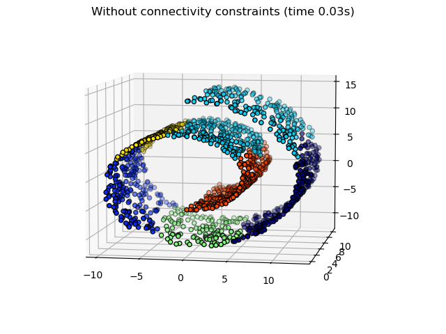
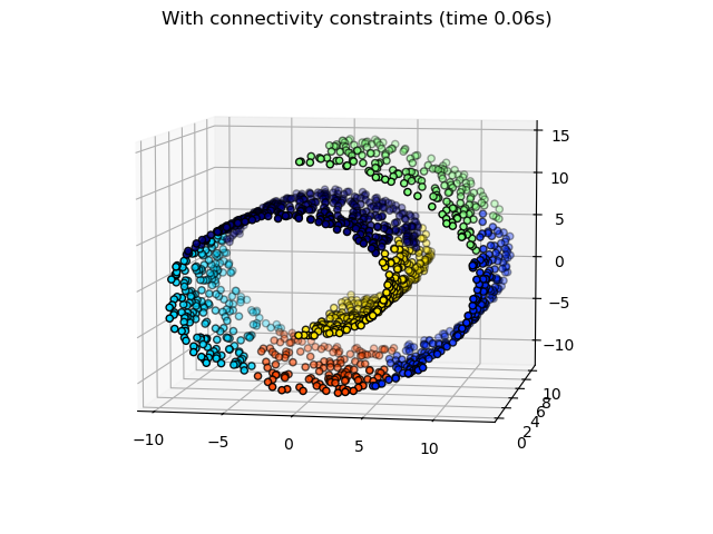
In a first step, the hierarchical clustering is performed without connectivity constraints on the structure and is solely based on distance, whereas in a second step the clustering is restricted to the k-Nearest Neighbors graph: it’s a hierarchical clustering with structure prior.
Some of the clusters learned without connectivity constraints do not respect the structure of the swiss roll and extend across different folds of the manifolds. On the opposite, when opposing connectivity constraints, the clusters form a nice parcellation of the swiss roll.
Authors: The scikit-learn developers
SPDX-License-Identifier: BSD-3-Clause
import time as time
The following import is required
for 3D projection to work with matplotlib < 3.2
import mpl_toolkits.mplot3d # noqa: F401 import numpy as np
Generate data#
We start by generating the Swiss Roll dataset.
from sklearn.datasets import make_swiss_roll
n_samples = 1500 noise = 0.05 X, _ = make_swiss_roll(n_samples, noise=noise)
Make it thinner
X[:, 1] *= 0.5
Compute clustering#
We perform AgglomerativeClustering which comes under Hierarchical Clustering without any connectivity constraints.
from sklearn.cluster import AgglomerativeClustering
print("Compute unstructured hierarchical clustering...") st = time.time() ward = AgglomerativeClustering(n_clusters=6, linkage="ward").fit(X) elapsed_time = time.time() - st label = ward.labels_ print(f"Elapsed time: {elapsed_time:.2f}s") print(f"Number of points: {label.size}")
Compute unstructured hierarchical clustering... Elapsed time: 0.03s Number of points: 1500
Plot result#
Plotting the unstructured hierarchical clusters.
import matplotlib.pyplot as plt
fig1 = plt.figure() ax1 = fig1.add_subplot(111, projection="3d", elev=7, azim=-80) ax1.set_position([0, 0, 0.95, 1]) for l in np.unique(label): ax1.scatter( X[label == l, 0], X[label == l, 1], X[label == l, 2], color=plt.cm.jet(float(l) / np.max(label + 1)), s=20, edgecolor="k", ) _ = fig1.suptitle(f"Without connectivity constraints (time {elapsed_time:.2f}s)")
We are defining k-Nearest Neighbors with 10 neighbors#
Compute clustering#
We perform AgglomerativeClustering again with connectivity constraints.
print("Compute structured hierarchical clustering...") st = time.time() ward = AgglomerativeClustering( n_clusters=6, connectivity=connectivity, linkage="ward" ).fit(X) elapsed_time = time.time() - st label = ward.labels_ print(f"Elapsed time: {elapsed_time:.2f}s") print(f"Number of points: {label.size}")
Compute structured hierarchical clustering... Elapsed time: 0.06s Number of points: 1500
Plot result#
Plotting the structured hierarchical clusters.
fig2 = plt.figure() ax2 = fig2.add_subplot(121, projection="3d", elev=7, azim=-80) ax2.set_position([0, 0, 0.95, 1]) for l in np.unique(label): ax2.scatter( X[label == l, 0], X[label == l, 1], X[label == l, 2], color=plt.cm.jet(float(l) / np.max(label + 1)), s=20, edgecolor="k", ) fig2.suptitle(f"With connectivity constraints (time {elapsed_time:.2f}s)")
plt.show()
Total running time of the script: (0 minutes 0.354 seconds)
Related examples