dlhdl.Workflow.predict - Predict responses by using deployed network - MATLAB (original) (raw)
Class: dlhdl.Workflow
Namespace: dlhdl
Predict responses by using deployed network
Since R2020b
Syntax
Description
[Y](#mw%5Fbb0c5f48-628a-4d95-9958-8229190ea1bd) = predict([workflowObject](#mw%5F8ac5a323-829c-4862-bf28-2b03a6362ead%5Fsep%5Fmw%5F348d2c6b-da53-4e76-ac9f-682c2e359b46),[images](#mw%5F169a4766-a257-49f0-85a3-ae29ea68a6af)) predicts responses for the image data, images, by using the deep learning network specified in the dlhdl.Workflow object,workflowObject.
[Y](#mw%5Fbb0c5f48-628a-4d95-9958-8229190ea1bd) = predict([workflowObject](#mw%5F8ac5a323-829c-4862-bf28-2b03a6362ead%5Fsep%5Fmw%5F348d2c6b-da53-4e76-ac9f-682c2e359b46),[X1,...,XN](#mw%5F5cfa6545-1eb5-44ec-a3ce-2bf7b4f5affb)) predicts the responses for the data in the numeric or cell arrays X1, …, XN for the multi-input network specified in theNetwork argument of the workflowObject. The input XN corresponds to theworkflowObject.Network.InputNames(N).
[[Y1,...,YM](#mw%5F5158af5f-66ca-4232-ae93-0251c6378fde)] = predict(___) predicts responses for the M outputs of a multi-output network using any of the previous input arguments. The output YM corresponds to the output of the network specified inworkflowObject.Network.OutputNames(M).
[[Y](#mw%5Fbb0c5f48-628a-4d95-9958-8229190ea1bd),[performance](#mw%5F038f887e-f25a-48d7-a08f-5161c1452e17)] = predict(___,[Name,Value](#namevaluepairarguments)) predicts the responses with one or more arguments specified by optional name-value pair arguments.
Input Arguments
Deep learning network deployment options, specified as adlhdl.Workflow object.
Input image, specified as a numeric array, cell array or formatteddlarray object. The numeric arrays can be 3-D or 4-D arrays. For 4-D arrays, the fourth dimension is the number of input images. If one of the members of the numeric array has four dimensions, then the other members of the numeric arrays must have four dimensions as well, with the value of the fourth dimension being the same for all members.
Data Types: single | int8
Numeric or cell arrays for networks with multiple inputs, specified as a numeric array or cell array.
For multiple inputs to image prediction networks, the format of the predictors must match the formats described in the images argument descriptions.
Data Types: single | double | int8 | int16 | int32 | int64 | uint8 | uint16 | uint32 | uint64
Name-Value Arguments
Specify optional pairs of arguments asName1=Value1,...,NameN=ValueN, where Name is the argument name and Value is the corresponding value. Name-value arguments must appear after other arguments, but the order of the pairs does not matter.
Before R2021a, use commas to separate each name and value, and enclose Name in quotes.
Flag to return profiling results for the deep learning network deployed to the target board, specified as "off" or "on".
Example: Profile = "on"
Option to keep the internal states so that you can perform predictions on a recurrent neural network (RNN) like long short-term memory (LSTM) layer and gated recurrent unit (GRU) layer networks and update the deployed network state, specified as a logical value. By default, the predict method resets the network state when performing a prediction on an RNN. To retain the network state, setKeepState to true.
Example: KeepState = true
Data Types: logical
The timeout property specifies the amount of time (in seconds) to wait for a prediction result to be returned from hardware.
Example: timeout = 20
Output Arguments
Predicted responses, returned as a numeric array. The format ofY depends on the type of task.
| Task | Format |
|---|---|
| 2-D image regression | _h_-by-_w_-by-c_-by-N numeric array, where h, w, and_c are the height, width, and number of channels of the images, respectively, and N is the number of images |
| 3-D image regression | _h_-by-_w_-by-_d_-by-c_-by-N numeric array, where h, w,d, and c are the height, width, depth, and number of channels of the images, respectively, and_N is the number of images |
| Sequence-to-one regression | N_-by-R matrix, where_N is the number of sequences and R is the number of responses |
| Sequence-to-sequence regression | N_-by-R matrix, where_N is the number of sequences and R is the number of responses |
| Feature regression | N_-by-R matrix, where_N is the number of observations and R is the number of responses |
For sequence-to-sequence regression problems with one observation,images can be a matrix. In this case, Y is a matrix of responses.
If the output layer of the network is a classification layer, thenY is the predicted classification scores. This table describes the format of the scores for classification tasks.
| Task | Format |
|---|---|
| Image classification | N_-by-K matrix, where_N is the number of observations and K is the number of classes |
| Sequence-to-label classification | |
| Feature classification |
Predicted scores or responses of networks with multiple outputs, returned as numeric arrays.
Each output Yj corresponds to the network outputnet.OutputNames(j) and has format as described in theY output argument.
Deployed network performance data, returned as an_N_-by-5 table, where_N_ is the number of layers in the network. This method returns performance only when the Profile name-value argument is set to 'on'. To learn about the data in the performance table, see Profile Inference Run.
Examples
This example shows how to deploy a custom trained network to detect pedestrians and bicyclists based on their micro-Doppler signatures. This network is taken from the Pedestrian and Bicyclist Classification Using Deep Learning example from the Phased Array Toolbox. For more details on network training and input data, see Pedestrian and Bicyclist Classification Using Deep Learning (Radar Toolbox).
Prerequisites
- Zynq® UltraScale+™ MPSoC ZCU102 Evaluation Kit
The data files used in this example are:
- The MAT File
trainedNetBicPed.matcontains a model trained on training data settrainDataNoCarand its label settrainLabelNoCar. - The MAT File
testDataBicPed.matcontains the test data settestDataNoCarand its label settestLabelNoCar.
Load Data and Network
Load the pretrained network. Load test data and its labels.
load('trainedNetBicPed.mat','trainedNetNoCar') load('testDataBicPed.mat')
View the layers of the pre-trained network:
deepNetworkDesigner(trainedNetNoCar);
Set Up HDL Toolpath
Set up the path to your installed Xilinx® Vivado® Design Suite 2023.1 executable if it is not already set up. For example, to set the toolpath, enter:
% hdlsetuptoolpath('ToolName', 'Xilinx Vivado','ToolPath', 'C:\Vivado\2023.1\bin');
Create Target Object
Create a target object for your target device with a vendor name and an interface to connect your target device to the host computer. Interface options are JTAG (default) and Ethernet. Vendor options are Intel or Xilinx. Use the installed Xilinx Vivado Design Suite over an Ethernet connection to program the device.
hT = dlhdl.Target('Xilinx', 'Interface', 'Ethernet');
Create Workflow Object
Create an object of the dlhdl.Workflow class. When you create the object, specify the network and the bitstream name. Specify the saved pre-trained network, trainedNetNoCar, as the network. Make sure the bitstream name matches the data type and the FPGA board that you are targeting. In this example, the target FPGA board is the Zynq UltraScale+ MPSoC ZCU102 board. The bitstream uses a single data type.
hW = dlhdl.Workflow('Network', trainedNetNoCar, 'Bitstream', 'zcu102_single', 'Target', hT);
Compile trainedNetNoCar Network
To compile the trainedNetNoCar network, run the compile function of the dlhdl.Workflow object.
Compiling network for Deep Learning FPGA prototyping ...
Targeting FPGA bitstream zcu102_single.
An output layer called 'Output1_softmax' of type 'nnet.cnn.layer.RegressionOutputLayer' has been added to the provided network. This layer performs no operation during prediction and thus does not affect the output of the network.
Optimizing network: Fused 'nnet.cnn.layer.BatchNormalizationLayer' into 'nnet.cnn.layer.Convolution2DLayer'
The network includes the following layers:
 1   'imageinput'        Image Input           400×144×1 images                                                 (SW Layer)
 2   'conv_1'            2-D Convolution       16 10×10×1 convolutions with stride [1  1] and padding 'same'    (HW Layer)
 3   'relu_1'            ReLU                  ReLU                                                             (HW Layer)
 4   'maxpool_1'         2-D Max Pooling       10×10 max pooling with stride [2  2] and padding [0  0  0  0]    (HW Layer)
 5   'conv_2'            2-D Convolution       32 5×5×16 convolutions with stride [1  1] and padding 'same'     (HW Layer)
 6   'relu_2'            ReLU                  ReLU                                                             (HW Layer)
 7   'maxpool_2'         2-D Max Pooling       10×10 max pooling with stride [2  2] and padding [0  0  0  0]    (HW Layer)
 8   'conv_3'            2-D Convolution       32 5×5×32 convolutions with stride [1  1] and padding 'same'     (HW Layer)
 9   'relu_3'            ReLU                  ReLU                                                             (HW Layer)
10   'maxpool_3'         2-D Max Pooling       10×10 max pooling with stride [2  2] and padding [0  0  0  0]    (HW Layer)
11   'conv_4'            2-D Convolution       32 5×5×32 convolutions with stride [1  1] and padding 'same'     (HW Layer)
12   'relu_4'            ReLU                  ReLU                                                             (HW Layer)
13   'maxpool_4'         2-D Max Pooling       5×5 max pooling with stride [2  2] and padding [0  0  0  0]      (HW Layer)
14   'conv_5'            2-D Convolution       32 5×5×32 convolutions with stride [1  1] and padding 'same'     (HW Layer)
15   'relu_5'            ReLU                  ReLU                                                             (HW Layer)
16   'avgpool2d'         2-D Average Pooling   2×2 average pooling with stride [2  2] and padding [0  0  0  0]  (HW Layer)
17   'fc'                Fully Connected       5 fully connected layer                                          (HW Layer)
18   'softmax'           Softmax               softmax                                                          (SW Layer)
19   'Output1_softmax'   Regression Output     mean-squared-error                                               (SW Layer)
Notice: The layer 'imageinput' with type 'nnet.cnn.layer.ImageInputLayer' is implemented in software.
Notice: The layer 'softmax' with type 'nnet.cnn.layer.SoftmaxLayer' is implemented in software.
Notice: The layer 'Output1_softmax' with type 'nnet.cnn.layer.RegressionOutputLayer' is implemented in software.
Compiling layer group: conv_1>>relu_5 ...
Compiling layer group: conv_1>>relu_5 ... complete.
Compiling layer group: avgpool2d ...
Compiling layer group: avgpool2d ... complete.
Compiling layer group: fc ...
Compiling layer group: fc ... complete.
Allocating external memory buffers:
      offset_name          offset_address    allocated_space
_______________________    ______________    ________________

"InputDataOffset"           "0x00000000"     "26.4 MB"
"OutputResultOffset"        "0x01a5e000"     "4.0 kB"
"SchedulerDataOffset"       "0x01a5f000"     "72.0 kB"
"SystemBufferOffset"        "0x01a71000"     "7.1 MB"
"InstructionDataOffset"     "0x0217e000"     "1020.0 kB"
"ConvWeightDataOffset"      "0x0227d000"     "888.0 kB"
"FCWeightDataOffset"        "0x0235b000"     "24.0 kB"
"EndOffset"                 "0x02361000"     "Total: 35.4 MB"
Network compilation complete.
Program the Bitstream onto FPGA and Download Network Weights
To deploy the network on the Zynq UltraScale+ MPSoC ZCU102 hardware, run the deploy function of the dlhdl.Workflow object. This function uses the output of the compile function to program the FPGA board by using the programming file. The function also downloads the network weights and biases. The deploy function checks for the Xilinx Vivado tool and the supported tool version. It then starts programming the FPGA device by using the bitstream, displays progress messages and the time it takes to deploy the network.
Programming FPGA Bitstream using Ethernet...
Attempting to connect to the hardware board at 192.168.1.101...
Connection successful
Programming FPGA device on Xilinx SoC hardware board at 192.168.1.101...
Attempting to connect to the hardware board at 192.168.1.101...
Connection successful
Copying FPGA programming files to SD card...
Setting FPGA bitstream and devicetree for boot...
Copying Bitstream zcu102_single.bit to /mnt/hdlcoder_rd
Set Bitstream to hdlcoder_rd/zcu102_single.bit
Copying Devicetree devicetree_dlhdl.dtb to /mnt/hdlcoder_rd
Set Devicetree to hdlcoder_rd/devicetree_dlhdl.dtb
Set up boot for Reference Design: 'AXI-Stream DDR Memory Access : 3-AXIM'
Programming done. The system will now reboot for persistent changes to take effect.
Rebooting Xilinx SoC at 192.168.1.101...
Reboot may take several seconds...
Attempting to connect to the hardware board at 192.168.1.101...
Connection successful
Programming the FPGA bitstream has been completed successfully.
Loading weights to Conv Processor.
Conv Weights loaded. Current time is 19-Jun-2024 17:04:03
Loading weights to FC Processor.
FC Weights loaded. Current time is 19-Jun-2024 17:04:03
Run Predictions on Micro-Doppler Signatures
Classify one input from the sample test data set by using the predict function of the dlhdl.Workflow object and display the label. The inputs to the network correspond to the sonograms of the micro-Doppler signatures for a pedestrian or a bicyclist or a combination of both.
testImg = single(testDataNoCar(:, :, :, 1)); testLabel = testLabelNoCar(1);
% Get predictions from network on single test input testImg = dlarray(testImg, 'SSCB'); score = hW.predict(testImg, 'Profile', 'On')
Finished writing input activations.
Running single input activation.
          Deep Learning Processor Profiler Performance Results

               LastFrameLatency(cycles)   LastFrameLatency(seconds)       FramesNum      Total Latency     Frames/s
                     -------------             -------------              ---------        ---------       ---------
Network 9312021 0.04233 1 9312779 23.6 conv_1 4186343 0.01903 maxpool_1 1387467 0.00631 conv_2 1976965 0.00899 maxpool_2 604660 0.00275 conv_3 816212 0.00371 maxpool_3 121647 0.00055 conv_4 146400 0.00067 maxpool_4 18760 0.00009 conv_5 42908 0.00020 avgpool2d 7226 0.00003 fc 3391 0.00002
- The clock frequency of the DL processor is: 220MHz
score = 5(C) × 1(B) single dlarray
0.9956
0.0000
0.0000
0.0044
0.0000
[~, idx1] = max(score); predTestLabel = testLabelNoCar(1,1,1,idx1)
predTestLabel = categorical ped
Load five random images from the sample test data set and execute the predict function of the dlhdl.Workflow object to display the labels alongside the signatures. The predictions will happen at once since the input is concatenated along the fourth dimension.
numTestFrames = size(testDataNoCar, 4); numView = 5; listIndex = randperm(numTestFrames, numView); testImgBatch = single(testDataNoCar(:, :, :, listIndex)); testLabelBatch = testLabelNoCar(listIndex);
% Get predictions from network using DL HDL Toolbox on FPGA testImgBatch = dlarray(testImgBatch, 'SSCB'); [scores, speed] = hW.predict(testImgBatch, 'Profile', 'On');
Finished writing input activations.
Running in multi-frame mode with 5 inputs.
          Deep Learning Processor Profiler Performance Results

               LastFrameLatency(cycles)   LastFrameLatency(seconds)       FramesNum      Total Latency     Frames/s
                     -------------             -------------              ---------        ---------       ---------
Network 9314346 0.04234 5 46556877 23.6 conv_1 4188705 0.01904 maxpool_1 1387527 0.00631 conv_2 1976807 0.00899 maxpool_2 604685 0.00275 conv_3 815776 0.00371 maxpool_3 121686 0.00055 conv_4 146622 0.00067 maxpool_4 18760 0.00009 conv_5 43098 0.00020 avgpool2d 7234 0.00003 fc 3404 0.00002
- The clock frequency of the DL processor is: 220MHz
[~, idx2] = max(scores, [], 1); predTestLabelBatch = testLabelNoCar(1,1,1,idx2);
% Display the micro-doppler signatures along with the ground truth and % predictions. for k = 1:numView index = listIndex(k); imagesc(testDataNoCar(:, :, :, index)); axis xy xlabel('Time (s)') ylabel('Frequency (Hz)') title('Ground Truth: '+string(testLabelNoCar(index))+', Prediction FPGA: '+string(predTestLabelBatch(k))) drawnow; pause(3); end

The image shows the micro-Doppler signatures of two bicyclists (bic+bic) which is the ground truth. The ground truth is the classification of the image against which the network prediction is compared. The network prediction retrieved from the FPGA correctly predicts that the image has two bicyclists.
This example shows how to use Deep Learning HDL Toolbox™ to deploy a quantized deep convolutional neural network (CNN) to an FPGA. In the example you use the pretrained ResNet-18 CNN to perform transfer learning and quantization. You then deploy the quantized network and use MATLAB® to retrieve the prediction results.
ResNet-18 has been trained on over a million images and can classify images into 1000 object categories, such as keyboard, coffee mug, pencil, and many animals. The network has learned rich feature representations for a wide range of images. The network takes an image as input and outputs a label for the object in the image together with the probabilities for each of the object categories.
To perform classification on a new set of images, you fine-tune a pretrained ResNet-18 CNN by transfer learning. In transfer learning, you can take a pretrained network and use it as a starting point to learn a new task. Fine-tuning a network with transfer learning is usually much faster and easier than training a network with randomly initialized weights. You can quickly transfer learned features to a new task using a smaller number of training images.
Load Pretrained Network
Load the pretrained ResNet-18 network.
net = imagePretrainedNetwork("resnet18");
View the layers of the pretrained network.
deepNetworkDesigner(net);
The first layer, the image input layer, requires input images of size 227-by-227-by-3, where three is the number of color channels.
inputSize = net.Layers(1).InputSize;
Load Data
This example uses the MathWorks® MerchData data set. This is a small data set containing 75 images of MathWorks merchandise, belonging to five different classes (cap, cube, playing cards, screwdriver, and torch).
curDir = pwd; unzip('MerchData.zip'); imds = imageDatastore('MerchData', ... 'IncludeSubfolders',true, ... 'LabelSource','foldernames');
Specify Training and Validation Sets
Divide the data into training and validation data sets, so that 30% percent of the images go to the training data set and 70% of the images to the validation data set. splitEachLabel splits the datastore imds into two new datastores, imdsTrain and imdsValidation.
[imdsTrain,imdsValidation] = splitEachLabel(imds,0.7,'randomized');
Replace Final layers
To retrain ResNet-18 to classify new images, replace the last fully connected layer of the network. In ResNet-18 , this layer has the name 'fc1000'. The fully connected layer of the pretrained network net is configured for 1000 classes. This layer, fc1000 in ResNet-18, contains information on how to combine the features that the network extracts into class probabilities. The layer must be fine-tuned for the new classification problem. Extract all the layers, except the last layer, from the pretrained network.
numClasses = numel(categories(imdsTrain.Labels))
newLearnableLayer = fullyConnectedLayer(numClasses, ... 'Name','new_fc', ... 'WeightLearnRateFactor',10, ... 'BiasLearnRateFactor',10); net = replaceLayer(net,'fc1000',newLearnableLayer);
Prepare Data for Training
The network requires input images of size 224-by-224-by-3, but the images in the image datastores have different sizes. Use an augmented image datastore to automatically resize the training images. Specify additional augmentation operations to perform on the training images, such as randomly flipping the training images along the vertical axis and randomly translating them up to 30 pixels horizontally and vertically. Data augmentation helps prevent the network from overfitting and memorizing the exact details of the training images.
pixelRange = [-30 30]; imageAugmenter = imageDataAugmenter( ... 'RandXReflection',true, ... 'RandXTranslation',pixelRange, ... 'RandYTranslation',pixelRange);
To automatically resize the validation images without performing further data augmentation, use an augmented image datastore without specifying any additional preprocessing operations.
augimdsTrain = augmentedImageDatastore(inputSize(1:2),imdsTrain, ... 'DataAugmentation',imageAugmenter); augimdsValidation = augmentedImageDatastore(inputSize(1:2),imdsValidation);
Specify Training Options
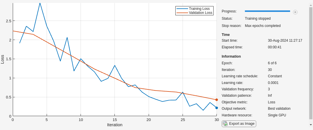
Specify the training options. For transfer learning, keep the features from the early layers of the pretrained network (the transferred layer weights). To slow down learning in the transferred layers, set the initial learning rate to a small value. Specify the mini-batch size and validation data. The software validates the network every ValidationFrequency iterations during training.
options = trainingOptions('sgdm', ... 'MiniBatchSize',10, ... 'MaxEpochs',6, ... 'InitialLearnRate',1e-4, ... 'Shuffle','every-epoch', ... 'ValidationData',augimdsValidation, ... 'ValidationFrequency',3, ... 'Verbose',false, ... 'Plots','training-progress');
Train Network
Train the network that consists of the transferred and new layers. By default, trainnet uses a GPU if one is available. Using this function on a GPU requires Parallel Computing Toolbox™ and a supported GPU device. For more information, see GPU Computing Requirements (Parallel Computing Toolbox). If a GPU is not available, the network uses a CPU (requires MATLAB Coder™ Interface for Deep Learning). You can also specify the execution environment by using the ExecutionEnvironment name-value argument of trainingOptions.
netTransfer = trainnet(augimdsTrain, net, 'crossentropy', options)
netTransfer = dlnetwork with properties:
     Layers: [70×1 nnet.cnn.layer.Layer]
Connections: [77×2 table]
 Learnables: [82×3 table]
      State: [40×3 table]
 InputNames: {'data'}
OutputNames: {'prob'}
Initialized: 1
View summary with summary.
Quantize Network
Quantize the network using the dlquantizer object. Set the target execution environment to FPGA.
dlquantObj = dlquantizer(netTransfer,'ExecutionEnvironment','FPGA');
Calibrate Quantized Network
Use the calibrate function to exercise the network with sample inputs and collect the range information. The calibrate function collects the dynamic ranges of the weights and biases in the convolution and fully connected layers of the network and the dynamic ranges of the activations in all layers of the network. The function returns the information as a table, in which each row contains range information for a learnable parameter of the quantized network.
calibrate(dlquantObj,augimdsTrain)
ans=94×5 table Optimized Layer Name Network Layer Name Learnables / Activations MinValue MaxValue __________________________ __________________ ________________________ ________ ________
{'conv1_Weights'         }    {'conv1'         }           "Weights"            -0.64526    0.89818
{'conv1_Bias'            }    {'conv1'         }           "Bias"               -0.64035    0.68777
{'res2a_branch2a_Weights'}    {'res2a_branch2a'}           "Weights"            -0.39021    0.33934
{'res2a_branch2a_Bias'   }    {'res2a_branch2a'}           "Bias"               -0.79958     1.2763
{'res2a_branch2b_Weights'}    {'res2a_branch2b'}           "Weights"            -0.75631    0.57786
{'res2a_branch2b_Bias'   }    {'res2a_branch2b'}           "Bias"                -1.3255     1.7421
{'res2b_branch2a_Weights'}    {'res2b_branch2a'}           "Weights"            -0.31048    0.33465
{'res2b_branch2a_Bias'   }    {'res2b_branch2a'}           "Bias"                -1.1135     1.4752
{'res2b_branch2b_Weights'}    {'res2b_branch2b'}           "Weights"             -1.1498    0.93351
{'res2b_branch2b_Bias'   }    {'res2b_branch2b'}           "Bias"               -0.84473     1.2549
{'res3a_branch2a_Weights'}    {'res3a_branch2a'}           "Weights"            -0.19053    0.24578
{'res3a_branch2a_Bias'   }    {'res3a_branch2a'}           "Bias"               -0.53824    0.68652
{'res3a_branch2b_Weights'}    {'res3a_branch2b'}           "Weights"            -0.54176    0.73187
{'res3a_branch2b_Bias'   }    {'res3a_branch2b'}           "Bias"               -0.68422     1.1596
{'res3a_branch1_Weights' }    {'res3a_branch1' }           "Weights"            -0.61816    0.95464
{'res3a_branch1_Bias'    }    {'res3a_branch1' }           "Bias"               -0.95381    0.77789
⋮**Define FPGA Board Interface
Define the target FPGA board programming interface by using the dlhdl.Target object. Create a programming interface with custom name for your target device and an Ethernet interface to connect the target device to the host computer.
hTarget = dlhdl.Target('Xilinx','Interface','Ethernet');
Prepare Network for Deployment
Prepare the network for deployment by creating a dlhdl.Workflow object. Specify the network and bitstream name. Ensure that the bitstream name matches the data type and the FPGA board that you are targeting. In this example, the target FPGA board is the Xilinx® Zynq® UltraScale+™ MPSoC ZCU102 board and the bitstream uses the int8 data type.
hW = dlhdl.Workflow(Network=dlquantObj,Bitstream='zcu102_int8',Target=hTarget);
Compile Network
Run the compile method of the dlhdl.Workflow object to compile the network and generate the instructions, weights, and biases for deployment.
dn = compile(hW,'InputFrameNumberLimit',15)
Compiling network for Deep Learning FPGA prototyping ...
Targeting FPGA bitstream zcu102_int8.
An output layer called 'Output1_prob' of type 'nnet.cnn.layer.RegressionOutputLayer' has been added to the provided network. This layer performs no operation during prediction and thus does not affect the output of the network.
Optimizing network: Fused 'nnet.cnn.layer.BatchNormalizationLayer' into 'nnet.cnn.layer.Convolution2DLayer'
The network includes the following layers:
Notice: The layer 'data' with type 'nnet.cnn.layer.ImageInputLayer' is implemented in software.
Notice: The layer 'prob' with type 'nnet.cnn.layer.SoftmaxLayer' is implemented in software.
Notice: The layer 'Output1_prob' with type 'nnet.cnn.layer.RegressionOutputLayer' is implemented in software.
Compiling layer group: conv1>>pool1 ...
Compiling layer group: conv1>>pool1 ... complete.
Compiling layer group: res2a_branch2a>>res2a_branch2b ...
Compiling layer group: res2a_branch2a>>res2a_branch2b ... complete.
Compiling layer group: res2b_branch2a>>res2b_branch2b ...
Compiling layer group: res2b_branch2a>>res2b_branch2b ... complete.
Compiling layer group: res3a_branch1 ...
Compiling layer group: res3a_branch1 ... complete.
Compiling layer group: res3a_branch2a>>res3a_branch2b ...
Compiling layer group: res3a_branch2a>>res3a_branch2b ... complete.
Compiling layer group: res3b_branch2a>>res3b_branch2b ...
Compiling layer group: res3b_branch2a>>res3b_branch2b ... complete.
Compiling layer group: res4a_branch1 ...
Compiling layer group: res4a_branch1 ... complete.
Compiling layer group: res4a_branch2a>>res4a_branch2b ...
Compiling layer group: res4a_branch2a>>res4a_branch2b ... complete.
Compiling layer group: res4b_branch2a>>res4b_branch2b ...
Compiling layer group: res4b_branch2a>>res4b_branch2b ... complete.
Compiling layer group: res5a_branch1 ...
Compiling layer group: res5a_branch1 ... complete.
Compiling layer group: res5a_branch2a>>res5a_branch2b ...
Compiling layer group: res5a_branch2a>>res5a_branch2b ... complete.
Compiling layer group: res5b_branch2a>>res5b_branch2b ...
Compiling layer group: res5b_branch2a>>res5b_branch2b ... complete.
Compiling layer group: pool5 ...
Compiling layer group: pool5 ... complete.
Compiling layer group: new_fc ...
Compiling layer group: new_fc ... complete.
Allocating external memory buffers:
      offset_name          offset_address    allocated_space
_______________________    ______________    ________________

"InputDataOffset"           "0x00000000"     "5.7 MB"
"OutputResultOffset"        "0x005be000"     "4.0 kB"
"SchedulerDataOffset"       "0x005bf000"     "712.0 kB"
"SystemBufferOffset"        "0x00671000"     "1.6 MB"
"InstructionDataOffset"     "0x007fe000"     "1.2 MB"
"ConvWeightDataOffset"      "0x00936000"     "13.5 MB"
"FCWeightDataOffset"        "0x016ab000"     "12.0 kB"
"EndOffset"                 "0x016ae000"     "Total: 22.7 MB"
Network compilation complete.
dn = struct with fields: weights: [1×1 struct] instructions: [1×1 struct] registers: [1×1 struct] syncInstructions: [1×1 struct] constantData: {} ddrInfo: [1×1 struct] resourceTable: [6×2 table]
Program Bitstream onto FPGA and Download Network Weights
To deploy the network on the Xilinx ZCU102 hardware, run the deploy function of the dlhdl.Workflow object. This function uses the output of the compile function to program the FPGA board by using the programming file. It also downloads the network weights and biases. The deploy function starts programming the FPGA device, displays progress messages, and the time it takes to deploy the network.
Programming FPGA Bitstream using Ethernet...
Attempting to connect to the hardware board at 172.21.88.150...
Connection successful
Programming FPGA device on Xilinx SoC hardware board at 172.21.88.150...
Attempting to connect to the hardware board at 172.21.88.150...
Connection successful
Copying FPGA programming files to SD card...
Setting FPGA bitstream and devicetree for boot...
Copying Bitstream zcu102_int8.bit to /mnt/hdlcoder_rd
Set Bitstream to hdlcoder_rd/zcu102_int8.bit
Copying Devicetree devicetree_dlhdl.dtb to /mnt/hdlcoder_rd
Set Devicetree to hdlcoder_rd/devicetree_dlhdl.dtb
Set up boot for Reference Design: 'AXI-Stream DDR Memory Access : 3-AXIM'
Programming done. The system will now reboot for persistent changes to take effect.
Rebooting Xilinx SoC at 172.21.88.150...
Reboot may take several seconds...
Attempting to connect to the hardware board at 172.21.88.150...
Connection successful
Programming the FPGA bitstream has been completed successfully.
Loading weights to Conv Processor.
Conv Weights loaded. Current time is 30-Aug-2024 11:31:45
Loading weights to FC Processor.
FC Weights loaded. Current time is 30-Aug-2024 11:31:45
Test Network
Load the example image.
imgFile = fullfile(pwd,'MathWorks_cube_0.jpg'); inputImg = imresize(imread(imgFile),[224 224]); imshow(inputImg)
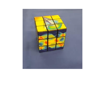
Classify the image on the FPGA by using the predict method of the dlhdl.Workflow object and display the results.
inputImg = dlarray(single(inputImg), 'SSCB'); [prediction,speed] = predict(hW,inputImg,'Profile','on');
Finished writing input activations.
Running single input activation.
          Deep Learning Processor Profiler Performance Results

               LastFrameLatency(cycles)   LastFrameLatency(seconds)       FramesNum      Total Latency     Frames/s
                     -------------             -------------              ---------        ---------       ---------
Network 7405555 0.02962 1 7408123 33.7 conv1 1115422 0.00446 pool1 200956 0.00080 res2a_branch2a 270504 0.00108 res2a_branch2b 270422 0.00108 res2a 109005 0.00044 res2b_branch2a 270206 0.00108 res2b_branch2b 270217 0.00108 res2b 109675 0.00044 res3a_branch1 155444 0.00062 res3a_branch2a 156720 0.00063 res3a_branch2b 245246 0.00098 res3a 54876 0.00022 res3b_branch2a 245640 0.00098 res3b_branch2b 245443 0.00098 res3b 55736 0.00022 res4a_branch1 135533 0.00054 res4a_branch2a 136768 0.00055 res4a_branch2b 238039 0.00095 res4a 27602 0.00011 res4b_branch2a 237950 0.00095 res4b_branch2b 238645 0.00095 res4b 27792 0.00011 res5a_branch1 324200 0.00130 res5a_branch2a 326074 0.00130 res5a_branch2b 623097 0.00249 res5a 13961 0.00006 res5b_branch2a 623607 0.00249 res5b_branch2b 624000 0.00250 res5b 13621 0.00005 pool5 36826 0.00015 new_fc 2141 0.00001
- The clock frequency of the DL processor is: 250MHz
scores2label(prediction,categories(imdsTrain.Labels))
ans = categorical MathWorks Cube
Performance Comparison
Compare the performance of the quantized network to the performance of the single data type network.
optionsFPGA = dlquantizationOptions('Bitstream','zcu102_int8','Target',hTarget, 'MetricFcn', {@(x)computeClassificationAccuracy(x,imdsValidation)}); predictionFPGA = validate(dlquantObj,imdsValidation,optionsFPGA)
Compiling network for Deep Learning FPGA prototyping ...
Targeting FPGA bitstream zcu102_int8.
An output layer called 'Output1_prob' of type 'nnet.cnn.layer.RegressionOutputLayer' has been added to the provided network. This layer performs no operation during prediction and thus does not affect the output of the network.
Optimizing network: Fused 'nnet.cnn.layer.BatchNormalizationLayer' into 'nnet.cnn.layer.Convolution2DLayer'
The network includes the following layers:
Notice: The layer 'data' with type 'nnet.cnn.layer.ImageInputLayer' is implemented in software.
Notice: The layer 'prob' with type 'nnet.cnn.layer.SoftmaxLayer' is implemented in software.
Notice: The layer 'Output1_prob' with type 'nnet.cnn.layer.RegressionOutputLayer' is implemented in software.
Compiling layer group: conv1>>pool1 ...
Compiling layer group: conv1>>pool1 ... complete.
Compiling layer group: res2a_branch2a>>res2a_branch2b ...
Compiling layer group: res2a_branch2a>>res2a_branch2b ... complete.
Compiling layer group: res2b_branch2a>>res2b_branch2b ...
Compiling layer group: res2b_branch2a>>res2b_branch2b ... complete.
Compiling layer group: res3a_branch1 ...
Compiling layer group: res3a_branch1 ... complete.
Compiling layer group: res3a_branch2a>>res3a_branch2b ...
Compiling layer group: res3a_branch2a>>res3a_branch2b ... complete.
Compiling layer group: res3b_branch2a>>res3b_branch2b ...
Compiling layer group: res3b_branch2a>>res3b_branch2b ... complete.
Compiling layer group: res4a_branch1 ...
Compiling layer group: res4a_branch1 ... complete.
Compiling layer group: res4a_branch2a>>res4a_branch2b ...
Compiling layer group: res4a_branch2a>>res4a_branch2b ... complete.
Compiling layer group: res4b_branch2a>>res4b_branch2b ...
Compiling layer group: res4b_branch2a>>res4b_branch2b ... complete.
Compiling layer group: res5a_branch1 ...
Compiling layer group: res5a_branch1 ... complete.
Compiling layer group: res5a_branch2a>>res5a_branch2b ...
Compiling layer group: res5a_branch2a>>res5a_branch2b ... complete.
Compiling layer group: res5b_branch2a>>res5b_branch2b ...
Compiling layer group: res5b_branch2a>>res5b_branch2b ... complete.
Compiling layer group: pool5 ...
Compiling layer group: pool5 ... complete.
Compiling layer group: new_fc ...
Compiling layer group: new_fc ... complete.
Allocating external memory buffers:
      offset_name          offset_address    allocated_space
_______________________    ______________    ________________

"InputDataOffset"           "0x00000000"     "11.5 MB"
"OutputResultOffset"        "0x00b7c000"     "4.0 kB"
"SchedulerDataOffset"       "0x00b7d000"     "720.0 kB"
"SystemBufferOffset"        "0x00c31000"     "1.6 MB"
"InstructionDataOffset"     "0x00dbe000"     "1.2 MB"
"ConvWeightDataOffset"      "0x00ef6000"     "13.5 MB"
"FCWeightDataOffset"        "0x01c6b000"     "12.0 kB"
"EndOffset"                 "0x01c6e000"     "Total: 28.4 MB"
Network compilation complete.
FPGA bitstream programming has been skipped as the same bitstream is already loaded on the target FPGA.
Loading weights to Conv Processor.
Conv Weights loaded. Current time is 30-Aug-2024 11:33:06
Loading weights to FC Processor.
FC Weights loaded. Current time is 30-Aug-2024 11:33:06
Finished writing input activations.
Running single input activation.
Finished writing input activations.
Running single input activation.
Finished writing input activations.
Running single input activation.
Finished writing input activations.
Running single input activation.
Finished writing input activations.
Running single input activation.
Finished writing input activations.
Running single input activation.
Finished writing input activations.
Running single input activation.
Finished writing input activations.
Running single input activation.
Finished writing input activations.
Running single input activation.
Finished writing input activations.
Running single input activation.
Finished writing input activations.
Running single input activation.
Finished writing input activations.
Running single input activation.
Finished writing input activations.
Running single input activation.
Finished writing input activations.
Running single input activation.
Finished writing input activations.
Running single input activation.
Finished writing input activations.
Running single input activation.
Finished writing input activations.
Running single input activation.
Finished writing input activations.
Running single input activation.
Finished writing input activations.
Running single input activation.
Finished writing input activations.
Running single input activation.
An output layer called 'Output1_prob' of type 'nnet.cnn.layer.RegressionOutputLayer' has been added to the provided network. This layer performs no operation during prediction and thus does not affect the output of the network.
Optimizing network: Fused 'nnet.cnn.layer.BatchNormalizationLayer' into 'nnet.cnn.layer.Convolution2DLayer'
Notice: The layer 'data' of type 'ImageInputLayer' is split into an image input layer 'data', an addition layer 'data_norm_add', and a multiplication layer 'data_norm' for hardware normalization.
The network includes the following layers:
Notice: The layer 'prob' with type 'nnet.cnn.layer.SoftmaxLayer' is implemented in software.
Notice: The layer 'Output1_prob' with type 'nnet.cnn.layer.RegressionOutputLayer' is implemented in software.
          Deep Learning Processor Estimator Performance Results

               LastFrameLatency(cycles)   LastFrameLatency(seconds)       FramesNum      Total Latency     Frames/s
                     -------------             -------------              ---------        ---------       ---------
Network 23781318 0.10810 1 23781318 9.3 data_norm_add 268453 0.00122 data_norm 163081 0.00074 conv1 2164700 0.00984 pool1 515128 0.00234 res2a_branch2a 966477 0.00439 res2a_branch2b 966477 0.00439 res2a 268453 0.00122 res2b_branch2a 966477 0.00439 res2b_branch2b 966477 0.00439 res2b 268453 0.00122 res3a_branch1 541373 0.00246 res3a_branch2a 541261 0.00246 res3a_branch2b 920141 0.00418 res3a 134257 0.00061 res3b_branch2a 920141 0.00418 res3b_branch2b 920141 0.00418 res3b 134257 0.00061 res4a_branch1 505453 0.00230 res4a_branch2a 511309 0.00232 res4a_branch2b 909517 0.00413 res4a 67152 0.00031 res4b_branch2a 909517 0.00413 res4b_branch2b 909517 0.00413 res4b 67152 0.00031 res5a_branch1 1045581 0.00475 res5a_branch2a 1052749 0.00479 res5a_branch2b 2017485 0.00917 res5a 33582 0.00015 res5b_branch2a 2017485 0.00917 res5b_branch2b 2017485 0.00917 res5b 33582 0.00015 pool5 55746 0.00025 new_fc 2259 0.00001
- The clock frequency of the DL processor is: 220MHz
Finished writing input activations.
Running single input activation.
predictionFPGA = struct with fields: NumSamples: 20 MetricResults: [1×1 struct] Statistics: [2×7 table]
View the frames per second performance for the quantized network and single-data-type network. The quantized network has a performance of 33.8 frames per second compared to 9.3 frames per second for the single-data-type network. You can use quantization to improve your frames per second performance, however you could lose accuracy when you quantize your networks.
predictionFPGA.Statistics.FramesPerSecond
However, in this case you can observe the accuracy to be the same for both networks.
predictionFPGA.MetricResults.Result
ans=2×2 table NetworkImplementation MetricOutput _____________________ ____________
 {'Floating-Point'}          0.9
 {'Quantized'     }          0.9
Helper Functions
function accuracy = computeClassificationAccuracy(fpgaOutput, validationData) % Compute accuracy of FPGA result compared to the Deep Learning Toolbox.
% Copyright 2024 The MathWorks, Inc.
fpgaClassifications = scores2label(fpgaOutput, categories(validationData.Labels)); fpgaClassifications = reshape(fpgaClassifications, size(validationData.Labels));
accuracy = sum(fpgaClassifications == validationData.Labels)./numel(fpgaClassifications);
end
This example shows how to deploy a trained you only look once (YOLO) v3 object detector to a target FPGA board. You then use MATLAB® to retrieve the object classification from the FPGA board.
Compared to YOLO v2 networks, YOLO v3 networks have additional detection heads that help detect smaller objects.
Create YOLO v3 Detector Object
In this example, you use a pretrained YOLO v3 object detector. To construct and train a custom YOLO v3 detector, see Object Detection Using YOLO v3 Deep Learning (Computer Vision Toolbox).
Use the downloadPretrainedYOLOv3Detector function to generate a dlnetwork object. To get the code for this function, see the downloadPretrainedYOLOv3Detector Function section.
preTrainedDetector = downloadPretrainedYOLOv3Detector;
Downloaded pretrained detector
The generated network uses training data to estimate the anchor boxes, which help the detector learn to predict the boxes. For more information about anchor boxes, see Anchor Boxes for Object Detection (Computer Vision Toolbox). The downloadPretrainedYOLOv3Detector function creates this YOLO v3 network:
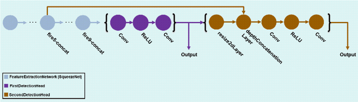
Load the Pretrained network
Extract the network from the pretrained YOLO v3 detector object.
yolov3Detector = preTrainedDetector; net = yolov3Detector.Network;
Extract the attributes of the network as variables.
anchorBoxes = yolov3Detector.AnchorBoxes; outputNames = yolov3Detector.Network.OutputNames; inputSize = yolov3Detector.InputSize; classNames = yolov3Detector.ClassNames;
Use the analyzeNetwork function to obtain information about the network layers. the function returns a graphical representation of the network that contains detailed parameter information for every layer in the network.
Define FPGA Board Interface
Define the target FPGA board programming interface by using the dlhdl.Target object. Create a programming interface with custom name for your target device and an Ethernet interface to connect the target device to the host computer.
hTarget = dlhdl.Target('Xilinx','Interface','Ethernet');
**Prepare Network for Deployment
Prepare the network for deployment by creating a dlhdl.Workflow object. Specify the network and bitstream name. Ensure that the bitstream name matches the data type and the FPGA board that you are targeting. In this example, the target FPGA board is the Xilinx® Zynq® UltraScale+™ MPSoC ZCU102 board and the bitstream uses the single data type.
hW = dlhdl.Workflow('Network',net,'Bitstream','zcu102_single','Target',hTarget);
Compile Network
Run the compile method of the dlhdl.Workflow object to compile the network and generate the instructions, weights, and biases for deployment.
Compiling network for Deep Learning FPGA prototyping ...
Targeting FPGA bitstream zcu102_single.
An output layer called 'Output1_customOutputConv1' of type 'nnet.cnn.layer.RegressionOutputLayer' has been added to the provided network. This layer performs no operation during prediction and thus does not affect the output of the network.
An output layer called 'Output2_customOutputConv2' of type 'nnet.cnn.layer.RegressionOutputLayer' has been added to the provided network. This layer performs no operation during prediction and thus does not affect the output of the network.
Optimizing network: Fused 'nnet.cnn.layer.BatchNormalizationLayer' into 'nnet.cnn.layer.Convolution2DLayer'
The network includes the following layers:
 1   'data'                        Image Input                    227×227×3 images                                                     (SW Layer)
 2   'conv1'                       2-D Convolution                64 3×3×3 convolutions with stride [2  2] and padding [0  0  0  0]    (HW Layer)
 3   'relu_conv1'                  ReLU                           ReLU                                                                 (HW Layer)
 4   'pool1'                       2-D Max Pooling                3×3 max pooling with stride [2  2] and padding [0  0  0  0]          (HW Layer)
 5   'fire2-squeeze1x1'            2-D Convolution                16 1×1×64 convolutions with stride [1  1] and padding [0  0  0  0]   (HW Layer)
 6   'fire2-relu_squeeze1x1'       ReLU                           ReLU                                                                 (HW Layer)
 7   'fire2-expand1x1'             2-D Convolution                64 1×1×16 convolutions with stride [1  1] and padding [0  0  0  0]   (HW Layer)
 8   'fire2-relu_expand1x1'        ReLU                           ReLU                                                                 (HW Layer)
 9   'fire2-expand3x3'             2-D Convolution                64 3×3×16 convolutions with stride [1  1] and padding [1  1  1  1]   (HW Layer)
10   'fire2-relu_expand3x3'        ReLU                           ReLU                                                                 (HW Layer)
11   'fire2-concat'                Depth concatenation            Depth concatenation of 2 inputs                                      (HW Layer)
12   'fire3-squeeze1x1'            2-D Convolution                16 1×1×128 convolutions with stride [1  1] and padding [0  0  0  0]  (HW Layer)
13   'fire3-relu_squeeze1x1'       ReLU                           ReLU                                                                 (HW Layer)
14   'fire3-expand1x1'             2-D Convolution                64 1×1×16 convolutions with stride [1  1] and padding [0  0  0  0]   (HW Layer)
15   'fire3-relu_expand1x1'        ReLU                           ReLU                                                                 (HW Layer)
16   'fire3-expand3x3'             2-D Convolution                64 3×3×16 convolutions with stride [1  1] and padding [1  1  1  1]   (HW Layer)
17   'fire3-relu_expand3x3'        ReLU                           ReLU                                                                 (HW Layer)
18   'fire3-concat'                Depth concatenation            Depth concatenation of 2 inputs                                      (HW Layer)
19   'pool3'                       2-D Max Pooling                3×3 max pooling with stride [2  2] and padding [0  1  0  1]          (HW Layer)
20   'fire4-squeeze1x1'            2-D Convolution                32 1×1×128 convolutions with stride [1  1] and padding [0  0  0  0]  (HW Layer)
21   'fire4-relu_squeeze1x1'       ReLU                           ReLU                                                                 (HW Layer)
22   'fire4-expand1x1'             2-D Convolution                128 1×1×32 convolutions with stride [1  1] and padding [0  0  0  0]  (HW Layer)
23   'fire4-relu_expand1x1'        ReLU                           ReLU                                                                 (HW Layer)
24   'fire4-expand3x3'             2-D Convolution                128 3×3×32 convolutions with stride [1  1] and padding [1  1  1  1]  (HW Layer)
25   'fire4-relu_expand3x3'        ReLU                           ReLU                                                                 (HW Layer)
26   'fire4-concat'                Depth concatenation            Depth concatenation of 2 inputs                                      (HW Layer)
27   'fire5-squeeze1x1'            2-D Convolution                32 1×1×256 convolutions with stride [1  1] and padding [0  0  0  0]  (HW Layer)
28   'fire5-relu_squeeze1x1'       ReLU                           ReLU                                                                 (HW Layer)
29   'fire5-expand1x1'             2-D Convolution                128 1×1×32 convolutions with stride [1  1] and padding [0  0  0  0]  (HW Layer)
30   'fire5-relu_expand1x1'        ReLU                           ReLU                                                                 (HW Layer)
31   'fire5-expand3x3'             2-D Convolution                128 3×3×32 convolutions with stride [1  1] and padding [1  1  1  1]  (HW Layer)
32   'fire5-relu_expand3x3'        ReLU                           ReLU                                                                 (HW Layer)
33   'fire5-concat'                Depth concatenation            Depth concatenation of 2 inputs                                      (HW Layer)
34   'pool5'                       2-D Max Pooling                3×3 max pooling with stride [2  2] and padding [0  1  0  1]          (HW Layer)
35   'fire6-squeeze1x1'            2-D Convolution                48 1×1×256 convolutions with stride [1  1] and padding [0  0  0  0]  (HW Layer)
36   'fire6-relu_squeeze1x1'       ReLU                           ReLU                                                                 (HW Layer)
37   'fire6-expand1x1'             2-D Convolution                192 1×1×48 convolutions with stride [1  1] and padding [0  0  0  0]  (HW Layer)
38   'fire6-relu_expand1x1'        ReLU                           ReLU                                                                 (HW Layer)
39   'fire6-expand3x3'             2-D Convolution                192 3×3×48 convolutions with stride [1  1] and padding [1  1  1  1]  (HW Layer)
40   'fire6-relu_expand3x3'        ReLU                           ReLU                                                                 (HW Layer)
41   'fire6-concat'                Depth concatenation            Depth concatenation of 2 inputs                                      (HW Layer)
42   'fire7-squeeze1x1'            2-D Convolution                48 1×1×384 convolutions with stride [1  1] and padding [0  0  0  0]  (HW Layer)
43   'fire7-relu_squeeze1x1'       ReLU                           ReLU                                                                 (HW Layer)
44   'fire7-expand1x1'             2-D Convolution                192 1×1×48 convolutions with stride [1  1] and padding [0  0  0  0]  (HW Layer)
45   'fire7-relu_expand1x1'        ReLU                           ReLU                                                                 (HW Layer)
46   'fire7-expand3x3'             2-D Convolution                192 3×3×48 convolutions with stride [1  1] and padding [1  1  1  1]  (HW Layer)
47   'fire7-relu_expand3x3'        ReLU                           ReLU                                                                 (HW Layer)
48   'fire7-concat'                Depth concatenation            Depth concatenation of 2 inputs                                      (HW Layer)
49   'fire8-squeeze1x1'            2-D Convolution                64 1×1×384 convolutions with stride [1  1] and padding [0  0  0  0]  (HW Layer)
50   'fire8-relu_squeeze1x1'       ReLU                           ReLU                                                                 (HW Layer)
51   'fire8-expand1x1'             2-D Convolution                256 1×1×64 convolutions with stride [1  1] and padding [0  0  0  0]  (HW Layer)
52   'fire8-relu_expand1x1'        ReLU                           ReLU                                                                 (HW Layer)
53   'fire8-expand3x3'             2-D Convolution                256 3×3×64 convolutions with stride [1  1] and padding [1  1  1  1]  (HW Layer)
54   'fire8-relu_expand3x3'        ReLU                           ReLU                                                                 (HW Layer)
55   'fire8-concat'                Depth concatenation            Depth concatenation of 2 inputs                                      (HW Layer)
56   'fire9-squeeze1x1'            2-D Convolution                64 1×1×512 convolutions with stride [1  1] and padding [0  0  0  0]  (HW Layer)
57   'fire9-relu_squeeze1x1'       ReLU                           ReLU                                                                 (HW Layer)
58   'fire9-expand1x1'             2-D Convolution                256 1×1×64 convolutions with stride [1  1] and padding [0  0  0  0]  (HW Layer)
59   'fire9-relu_expand1x1'        ReLU                           ReLU                                                                 (HW Layer)
60   'fire9-expand3x3'             2-D Convolution                256 3×3×64 convolutions with stride [1  1] and padding [1  1  1  1]  (HW Layer)
61   'fire9-relu_expand3x3'        ReLU                           ReLU                                                                 (HW Layer)
62   'fire9-concat'                Depth concatenation            Depth concatenation of 2 inputs                                      (HW Layer)
63   'customConv1'                 2-D Convolution                1024 3×3×512 convolutions with stride [1  1] and padding 'same'      (HW Layer)
64   'customRelu1'                 ReLU                           ReLU                                                                 (HW Layer)
65   'customOutputConv1'           2-D Convolution                18 1×1×1024 convolutions with stride [1  1] and padding 'same'       (HW Layer)
66   'featureConv2'                2-D Convolution                128 1×1×512 convolutions with stride [1  1] and padding 'same'       (HW Layer)
67   'featureRelu2'                ReLU                           ReLU                                                                 (HW Layer)
68   'Output1_customOutputConv1'   Regression Output              mean-squared-error                                                   (SW Layer)
69   'featureResize2'              dnnfpga.custom.Resize2DLayer   dnnfpga.custom.Resize2DLayer                                         (HW Layer)
70   'depthConcat2'                Depth concatenation            Depth concatenation of 2 inputs                                      (HW Layer)
71   'customConv2'                 2-D Convolution                256 3×3×384 convolutions with stride [1  1] and padding 'same'       (HW Layer)
72   'customRelu2'                 ReLU                           ReLU                                                                 (HW Layer)
73   'customOutputConv2'           2-D Convolution                18 1×1×256 convolutions with stride [1  1] and padding 'same'        (HW Layer)
74   'Output2_customOutputConv2'   Regression Output              mean-squared-error                                                   (SW Layer)
Notice: The layer 'data' with type 'nnet.cnn.layer.ImageInputLayer' is implemented in software.
Notice: The layer 'Output1_customOutputConv1' with type 'nnet.cnn.layer.RegressionOutputLayer' is implemented in software.
Notice: The layer 'Output2_customOutputConv2' with type 'nnet.cnn.layer.RegressionOutputLayer' is implemented in software.
Compiling layer group: conv1>>fire2-relu_squeeze1x1 ...
Compiling layer group: conv1>>fire2-relu_squeeze1x1 ... complete.
Compiling layer group: fire2-expand1x1>>fire2-relu_expand1x1 ...
Compiling layer group: fire2-expand1x1>>fire2-relu_expand1x1 ... complete.
Compiling layer group: fire2-expand3x3>>fire2-relu_expand3x3 ...
Compiling layer group: fire2-expand3x3>>fire2-relu_expand3x3 ... complete.
Compiling layer group: fire3-squeeze1x1>>fire3-relu_squeeze1x1 ...
Compiling layer group: fire3-squeeze1x1>>fire3-relu_squeeze1x1 ... complete.
Compiling layer group: fire3-expand1x1>>fire3-relu_expand1x1 ...
Compiling layer group: fire3-expand1x1>>fire3-relu_expand1x1 ... complete.
Compiling layer group: fire3-expand3x3>>fire3-relu_expand3x3 ...
Compiling layer group: fire3-expand3x3>>fire3-relu_expand3x3 ... complete.
Compiling layer group: pool3>>fire4-relu_squeeze1x1 ...
Compiling layer group: pool3>>fire4-relu_squeeze1x1 ... complete.
Compiling layer group: fire4-expand1x1>>fire4-relu_expand1x1 ...
Compiling layer group: fire4-expand1x1>>fire4-relu_expand1x1 ... complete.
Compiling layer group: fire4-expand3x3>>fire4-relu_expand3x3 ...
Compiling layer group: fire4-expand3x3>>fire4-relu_expand3x3 ... complete.
Compiling layer group: fire5-squeeze1x1>>fire5-relu_squeeze1x1 ...
Compiling layer group: fire5-squeeze1x1>>fire5-relu_squeeze1x1 ... complete.
Compiling layer group: fire5-expand1x1>>fire5-relu_expand1x1 ...
Compiling layer group: fire5-expand1x1>>fire5-relu_expand1x1 ... complete.
Compiling layer group: fire5-expand3x3>>fire5-relu_expand3x3 ...
Compiling layer group: fire5-expand3x3>>fire5-relu_expand3x3 ... complete.
Compiling layer group: pool5>>fire6-relu_squeeze1x1 ...
Compiling layer group: pool5>>fire6-relu_squeeze1x1 ... complete.
Compiling layer group: fire6-expand1x1>>fire6-relu_expand1x1 ...
Compiling layer group: fire6-expand1x1>>fire6-relu_expand1x1 ... complete.
Compiling layer group: fire6-expand3x3>>fire6-relu_expand3x3 ...
Compiling layer group: fire6-expand3x3>>fire6-relu_expand3x3 ... complete.
Compiling layer group: fire7-squeeze1x1>>fire7-relu_squeeze1x1 ...
Compiling layer group: fire7-squeeze1x1>>fire7-relu_squeeze1x1 ... complete.
Compiling layer group: fire7-expand1x1>>fire7-relu_expand1x1 ...
Compiling layer group: fire7-expand1x1>>fire7-relu_expand1x1 ... complete.
Compiling layer group: fire7-expand3x3>>fire7-relu_expand3x3 ...
Compiling layer group: fire7-expand3x3>>fire7-relu_expand3x3 ... complete.
Compiling layer group: fire8-squeeze1x1>>fire8-relu_squeeze1x1 ...
Compiling layer group: fire8-squeeze1x1>>fire8-relu_squeeze1x1 ... complete.
Compiling layer group: fire8-expand1x1>>fire8-relu_expand1x1 ...
Compiling layer group: fire8-expand1x1>>fire8-relu_expand1x1 ... complete.
Compiling layer group: fire8-expand3x3>>fire8-relu_expand3x3 ...
Compiling layer group: fire8-expand3x3>>fire8-relu_expand3x3 ... complete.
Compiling layer group: fire9-squeeze1x1>>fire9-relu_squeeze1x1 ...
Compiling layer group: fire9-squeeze1x1>>fire9-relu_squeeze1x1 ... complete.
Compiling layer group: fire9-expand1x1>>fire9-relu_expand1x1 ...
Compiling layer group: fire9-expand1x1>>fire9-relu_expand1x1 ... complete.
Compiling layer group: fire9-expand3x3>>fire9-relu_expand3x3 ...
Compiling layer group: fire9-expand3x3>>fire9-relu_expand3x3 ... complete.
Compiling layer group: customConv1>>customOutputConv1 ...
Compiling layer group: customConv1>>customOutputConv1 ... complete.
Compiling layer group: featureConv2>>featureRelu2 ...
Compiling layer group: featureConv2>>featureRelu2 ... complete.
Compiling layer group: customConv2>>customOutputConv2 ...
Compiling layer group: customConv2>>customOutputConv2 ... complete.
Allocating external memory buffers:
      offset_name          offset_address     allocated_space
_______________________    ______________    _________________

"InputDataOffset"           "0x00000000"     "24.0 MB"
"OutputResultOffset"        "0x01800000"     "4.0 MB"
"SchedulerDataOffset"       "0x01c00000"     "4.0 MB"
"SystemBufferOffset"        "0x02000000"     "28.0 MB"
"InstructionDataOffset"     "0x03c00000"     "8.0 MB"
"ConvWeightDataOffset"      "0x04400000"     "104.0 MB"
"EndOffset"                 "0x0ac00000"     "Total: 172.0 MB"
Network compilation complete.
Program Bitstream onto FPGA and Download Network Weights
To deploy the network on the Xilinx® Zynq® UltraScale+ MPSoC ZCU102 hardware, run the deploy method of the dlhdl.Workflow object. This method programs the FPGA board using the output of the compile method and the programming file, downloads the network weights and biases, displays progress messages, and the time it takes to deploy the network.
Programming FPGA Bitstream using Ethernet...
Attempting to connect to the hardware board at 192.168.1.101...
Connection successful
Programming FPGA device on Xilinx SoC hardware board at 192.168.1.101...
Copying FPGA programming files to SD card...
Setting FPGA bitstream and devicetree for boot...
Copying Bitstream zcu102_single.bit to /mnt/hdlcoder_rd
Set Bitstream to hdlcoder_rd/zcu102_single.bit
Copying Devicetree devicetree_dlhdl.dtb to /mnt/hdlcoder_rd
Set Devicetree to hdlcoder_rd/devicetree_dlhdl.dtb
Set up boot for Reference Design: 'AXI-Stream DDR Memory Access : 3-AXIM'
Rebooting Xilinx SoC at 192.168.1.101...
Reboot may take several seconds...
Attempting to connect to the hardware board at 192.168.1.101...
Connection successful
Programming the FPGA bitstream has been completed successfully.
Loading weights to Conv Processor.
Conv Weights loaded. Current time is 27-Oct-2022 13:44:50
Test Network
Load the example image and convert the image into a dlarray. Then classify the image on the FPGA by using the predict method of the dlhdl.Workflow object and display the results.
img = imread('vehicle_image.jpg'); I = single(rescale(img)); I = imresize(I, yolov3Detector.InputSize(1:2)); dlX = dlarray(I,'SSC');
Store the output of each detection head of the network in the features variable. Pass features to the post-processing function processYOLOv3Output to combine the multiple outputs and compute the final results. To get the code for this function, see the processYOLOv3Output Function section.
features = cell(size(net.OutputNames')); [features{:}] = hW.predict(dlX, 'Profiler', 'on');
Finished writing input activations.
Running single input activation.
          Deep Learning Processor Profiler Performance Results

               LastFrameLatency(cycles)   LastFrameLatency(seconds)       FramesNum      Total Latency     Frames/s
                     -------------             -------------              ---------        ---------       ---------
Network 34469645 0.15668 1 34473970 6.4 conv1 673148 0.00306 pool1 509022 0.00231 fire2-squeeze1x1 308280 0.00140 fire2-expand1x1 305546 0.00139 fire2-expand3x3 305227 0.00139 fire3-squeeze1x1 628018 0.00285 fire3-expand1x1 305219 0.00139 fire3-expand3x3 305220 0.00139 pool3 286781 0.00130 fire4-squeeze1x1 264346 0.00120 fire4-expand1x1 264777 0.00120 fire4-expand3x3 264750 0.00120 fire5-squeeze1x1 749166 0.00341 fire5-expand1x1 264800 0.00120 fire5-expand3x3 264880 0.00120 pool5 219686 0.00100 fire6-squeeze1x1 195193 0.00089 fire6-expand1x1 145091 0.00066 fire6-expand3x3 145075 0.00066 fire7-squeeze1x1 290001 0.00132 fire7-expand1x1 144830 0.00066 fire7-expand3x3 145390 0.00066 fire8-squeeze1x1 369605 0.00168 fire8-expand1x1 245085 0.00111 fire8-expand3x3 245208 0.00111 fire9-squeeze1x1 490784 0.00223 fire9-expand1x1 244864 0.00111 fire9-expand3x3 245458 0.00112 customConv1 17592876 0.07997 customOutputConv1 952889 0.00433 featureConv2 913457 0.00415 featureResize2 57819 0.00026 customConv2 5600648 0.02546 customOutputConv2 526143 0.00239
- The clock frequency of the DL processor is: 220MHz
[bboxes, scores, labels] = processYOLOv3Output(anchorBoxes, inputSize, classNames, features, I); resultImage = insertObjectAnnotation(I,'rectangle',bboxes,scores); imshow(resultImage)
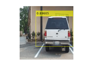
The FPGA returns a score prediction of 0.89605 with a bounding box drawn around the object in the image. The FPGA also returns a prediction of vehicle to the labels variable.
downloadPretrainedYOLOv3Detector Function
The downloadPretrainedYOLOv3Detector function to download the pretrained YOLO v3 detector network:
function detector = downloadPretrainedYOLOv3Detector if ~exist('yolov3SqueezeNetVehicleExample_21aSPKG.mat', 'file') if ~exist('yolov3SqueezeNetVehicleExample_21aSPKG.zip', 'file') zipFile = matlab.internal.examples.downloadSupportFile('vision/data', 'yolov3SqueezeNetVehicleExample_21aSPKG.zip'); copyfile(zipFile); end unzip('yolov3SqueezeNetVehicleExample_21aSPKG.zip'); end pretrained = load("yolov3SqueezeNetVehicleExample_21aSPKG.mat"); detector = pretrained.detector; disp('Downloaded pretrained detector'); end
processYOLOv3Output Function
The processYOLOv3Output function is attached as a helper file in this example's directory. This function converts the feature maps from multiple detection heads to bounding boxes, scores and labels. A code snippet of the function is shown below.
function [bboxes, scores, labels] = processYOLOv3Output(anchorBoxes, inputSize, classNames, features, img) % This function converts the feature maps from multiple detection heads to bounding boxes, scores and labels % processYOLOv3Output is C code generatable
% Breaks down the raw output from predict function into Confidence score, X, Y, Width, % Height and Class probabilities for each output from detection head predictions = iYolov3Transform(features, anchorBoxes);
% Initialize parameters for post-processing
inputSize2d = inputSize(1:2);
info.PreprocessedImageSize = inputSize2d(1:2);
info.ScaleX = size(img,1)/inputSize2d(1);
info.ScaleY = size(img,2)/inputSize2d(1);
params.MinSize = [1 1];
params.MaxSize = size(img(:,:,1));
params.Threshold = 0.5;
params.FractionDownsampling = 1;
params.DetectionInputWasBatchOfImages = false;
params.NetworkInputSize = inputSize;
params.DetectionPreprocessing = "none";
params.SelectStrongest = 1;
bboxes = [];
scores = [];
labels = [];
% Post-process the predictions to get bounding boxes, scores and labels [bboxes, scores, labels] = iPostprocessMultipleDetection(anchorBoxes, inputSize, classNames, predictions, info, params); end
function [bboxes, scores, labels] = iPostprocessMultipleDetection (anchorBoxes, inputSize, classNames, YPredData, info, params) % Post-process the predictions to get bounding boxes, scores and labels
% YpredData is a (x,8) cell array, where x = number of detection heads % Information in each column is: % column 1 -> confidence scores % column 2 to column 5 -> X offset, Y offset, Width, Height of anchor boxes % column 6 -> class probabilities % column 7-8 -> copy of width and height of anchor boxes
% Initialize parameters for post-processing classes = classNames; predictions = YPredData; extractPredictions = cell(size(predictions)); % Extract dlarray data for i = 1:size(extractPredictions,1) for j = 1:size(extractPredictions,2) extractPredictions{i,j} = extractdata(predictions{i,j}); end end
% Storing the values of columns 2 to 5 of extractPredictions % Columns 2 to 5 represent information about X-coordinate, Y-coordinate, Width and Height of predicted anchor boxes extractedCoordinates = cell(size(predictions,1),4); for i = 1:size(predictions,1) for j = 2:5 extractedCoordinates{i,j-1} = extractPredictions{i,j}; end end
% Convert predictions from grid cell coordinates to box coordinates. boxCoordinates = anchorBoxGenerator(anchorBoxes, inputSize, classNames, extractedCoordinates, params.NetworkInputSize); % Replace grid cell coordinates in extractPredictions with box coordinates for i = 1:size(YPredData,1) for j = 2:5 extractPredictions{i,j} = single(boxCoordinates{i,j-1}); end end
% 1. Convert bboxes from spatial to pixel dimension % 2. Combine the prediction from different heads. % 3. Filter detections based on threshold.
% Reshaping the matrices corresponding to confidence scores and bounding boxes detections = cell(size(YPredData,1),6); for i = 1:size(detections,1) for j = 1:5 detections{i,j} = reshapePredictions(extractPredictions{i,j}); end end % Reshaping the matrices corresponding to class probablities numClasses = repmat({numel(classes)},[size(detections,1),1]); for i = 1:size(detections,1) detections{i,6} = reshapeClasses(extractPredictions{i,6},numClasses{i,1}); end
% cell2mat converts the cell of matrices into one matrix, this combines the % predictions of all detection heads detections = cell2mat(detections);
% Getting the most probable class and corresponding index [classProbs, classIdx] = max(detections(:,6:end),[],2); detections(:,1) = detections(:,1).*classProbs; detections(:,6) = classIdx;
% Keep detections whose confidence score is greater than threshold. detections = detections(detections(:,1) >= params.Threshold,:);
[bboxes, scores, labels] = iPostProcessDetections(detections, classes, info, params); end
function [bboxes, scores, labels] = iPostProcessDetections(detections, classes, info, params) % Resizes the anchor boxes, filters anchor boxes based on size and apply % NMS to eliminate overlapping anchor boxes if ~isempty(detections)
% Obtain bounding boxes and class data for pre-processed image
scorePred = detections(:,1);
bboxesTmp = detections(:,2:5);
classPred = detections(:,6);
inputImageSize = ones(1,2);
inputImageSize(2) = info.ScaleX.*info.PreprocessedImageSize(2);
inputImageSize(1) = info.ScaleY.*info.PreprocessedImageSize(1);
% Resize boxes to actual image size.
scale = [inputImageSize(2) inputImageSize(1) inputImageSize(2) inputImageSize(1)];
bboxPred = bboxesTmp.*scale;
% Convert x and y position of detections from centre to top-left.
bboxPred = iConvertCenterToTopLeft(bboxPred);

% Filter boxes based on MinSize, MaxSize.
[bboxPred, scorePred, classPred] = filterBBoxes(params.MinSize, params.MaxSize, bboxPred, scorePred, classPred);

% Apply NMS to eliminate boxes having significant overlap
if params.SelectStrongest
    [bboxes, scores, classNames] = selectStrongestBboxMulticlass(bboxPred, scorePred, classPred ,...
        'RatioType', 'Union', 'OverlapThreshold', 0.4);
else
    bboxes = bboxPred;
    scores = scorePred;
    classNames = classPred;
end

% Limit width detections
detectionsWd = min((bboxes(:,1) + bboxes(:,3)),inputImageSize(1,2));
bboxes(:,3) = detectionsWd(:,1) - bboxes(:,1);

% Limit height detections
detectionsHt = min((bboxes(:,2) + bboxes(:,4)),inputImageSize(1,1));
bboxes(:,4) = detectionsHt(:,1) - bboxes(:,2);
bboxes(bboxes<1) = 1;

% Convert classId to classNames.
labels = categorical(classes,cellstr(classes));
labels = labels(classNames);
else % If detections are empty then bounding boxes, scores and labels should % be empty bboxes = zeros(0,4,'single'); scores = zeros(0,1,'single'); labels = categorical(classes); end end
function x = reshapePredictions(pred) % Reshapes the matrices corresponding to scores, X, Y, Width and Height to % make them compatible for combining the outputs of different detection % heads [h,w,c,n] = size(pred); x = reshape(pred,hwc,1,n); end
function x = reshapeClasses(pred,numClasses) % Reshapes the matrices corresponding to the class probabilities, to make it % compatible for combining the outputs of different detection heads [h,w,c,n] = size(pred); numAnchors = c/numClasses; x = reshape(pred,hw,numClasses,numAnchors,n); x = permute(x,[1,3,2,4]); [h,w,c,n] = size(x); x = reshape(x,hw,c,n); end
function bboxes = iConvertCenterToTopLeft(bboxes) % Convert x and y position of detections from centre to top-left. bboxes(:,1) = bboxes(:,1) - bboxes(:,3)/2 + 0.5; bboxes(:,2) = bboxes(:,2) - bboxes(:,4)/2 + 0.5; bboxes = floor(bboxes); bboxes(bboxes<1) = 1; end
function tiledAnchors = anchorBoxGenerator(anchorBoxes, inputSize, classNames,YPredCell,inputImageSize)
% Convert grid cell coordinates to box coordinates.
% Generate tiled anchor offset.
tiledAnchors = cell(size(YPredCell));
for i = 1:size(YPredCell,1)
anchors = anchorBoxes{i,:};
[h,w,,n] = size(YPredCell{i,1});
[tiledAnchors{i,2},tiledAnchors{i,1}] = ndgrid(0:h-1,0:w-1,1:size(anchors,1),1:n);
[,,tiledAnchors{i,3}] = ndgrid(0:h-1,0:w-1,anchors(:,2),1:n);
[,~,tiledAnchors{i,4}] = ndgrid(0:h-1,0:w-1,anchors(:,1),1:n);
end
for i = 1:size(YPredCell,1)
[h,w,,] = size(YPredCell{i,1});
tiledAnchors{i,1} = double((tiledAnchors{i,1} + YPredCell{i,1})./w);
tiledAnchors{i,2} = double((tiledAnchors{i,2} + YPredCell{i,2})./h);
tiledAnchors{i,3} = double((tiledAnchors{i,3}.*YPredCell{i,3})./inputImageSize(2));
tiledAnchors{i,4} = double((tiledAnchors{i,4}.*YPredCell{i,4})./inputImageSize(1));
end
end
function predictions = iYolov3Transform(YPredictions, anchorBoxes) % This function breaks down the raw output from predict function into Confidence score, X, Y, Width, % Height and Class probabilities for each output from detection head
predictions = cell(size(YPredictions,1),size(YPredictions,2) + 2);
for idx = 1:size(YPredictions,1) % Get the required info on feature size. numChannelsPred = size(YPredictions{idx},3); %number of channels in a feature map numAnchors = size(anchorBoxes{idx},1); %number of anchor boxes per grid numPredElemsPerAnchors = numChannelsPred/numAnchors; channelsPredIdx = 1:numChannelsPred; predictionIdx = ones([1,numAnchors.*5]);
% X positions.
startIdx = 1;
endIdx = numChannelsPred;
stride = numPredElemsPerAnchors;
predictions{idx,2} = YPredictions{idx}(:,:,startIdx:stride:endIdx,:);
predictionIdx = [predictionIdx startIdx:stride:endIdx];

% Y positions.
startIdx = 2;
endIdx = numChannelsPred;
stride = numPredElemsPerAnchors;
predictions{idx,3} = YPredictions{idx}(:,:,startIdx:stride:endIdx,:);
predictionIdx = [predictionIdx startIdx:stride:endIdx];

% Width.
startIdx = 3;
endIdx = numChannelsPred;
stride = numPredElemsPerAnchors;
predictions{idx,4} = YPredictions{idx}(:,:,startIdx:stride:endIdx,:);
predictionIdx = [predictionIdx startIdx:stride:endIdx];

% Height.
startIdx = 4;
endIdx = numChannelsPred;
stride = numPredElemsPerAnchors;
predictions{idx,5} = YPredictions{idx}(:,:,startIdx:stride:endIdx,:);
predictionIdx = [predictionIdx startIdx:stride:endIdx];

% Confidence scores.
startIdx = 5;
endIdx = numChannelsPred;
stride = numPredElemsPerAnchors;
predictions{idx,1} = YPredictions{idx}(:,:,startIdx:stride:endIdx,:);
predictionIdx = [predictionIdx startIdx:stride:endIdx];

% Class probabilities.
classIdx = setdiff(channelsPredIdx,predictionIdx);
predictions{idx,6} = YPredictions{idx}(:,:,classIdx,:);
end
for i = 1:size(predictions,1) predictions{i,7} = predictions{i,4}; predictions{i,8} = predictions{i,5}; end
% Apply activation to the predicted cell array % Apply sigmoid activation to columns 1-3 (Confidence score, X, Y) for i = 1:size(predictions,1) for j = 1:3 predictions{i,j} = sigmoid(predictions{i,j}); end end % Apply exponentiation to columns 4-5 (Width, Height) for i = 1:size(predictions,1) for j = 4:5 predictions{i,j} = exp(predictions{i,j}); end end % Apply sigmoid activation to column 6 (Class probabilities) for i = 1:size(predictions,1) for j = 6 predictions{i,j} = sigmoid(predictions{i,j}); end end end
function [bboxPred, scorePred, classPred] = filterBBoxes(minSize, maxSize, bboxPred, scorePred, classPred) % Filter boxes based on MinSize, MaxSize [bboxPred, scorePred, classPred] = filterSmallBBoxes(minSize, bboxPred, scorePred, classPred); [bboxPred, scorePred, classPred] = filterLargeBBoxes(maxSize, bboxPred, scorePred, classPred); end
function varargout = filterSmallBBoxes(minSize, varargin) % Filter boxes based on MinSize bboxes = varargin{1}; tooSmall = any((bboxes(:,[4 3]) < minSize),2); for ii = 1:numel(varargin) varargout{ii} = varargin{ii}(~tooSmall,:); end end
function varargout = filterLargeBBoxes(maxSize, varargin) % Filter boxes based on MaxSize bboxes = varargin{1}; tooBig = any((bboxes(:,[4 3]) > maxSize),2); for ii = 1:numel(varargin) varargout{ii} = varargin{ii}(~tooBig,:); end end
function m = cell2mat(c) % Converts the cell of matrices into one matrix by concatenating % the output corresponding to each feature map
elements = numel(c); % If number of elements is 0 return an empty array if elements == 0 m = []; return end % If number of elements is 1, return same element as matrix if elements == 1 if isnumeric(c{1}) || ischar(c{1}) || islogical(c{1}) || isstruct(c{1}) m = c{1}; return end end % Error out for unsupported cell content ciscell = iscell(c{1}); cisobj = isobject(c{1}); if cisobj || ciscell disp('CELL2MAT does not support cell arrays containing cell arrays or objects.'); end % If input is struct, extract field names of structure into a cell if isstruct(c{1}) cfields = cell(elements,1); for n = 1:elements cfields{n} = fieldnames(c{n}); end if ~isequal(cfields{:}) disp('The field names of each cell array element must be consistent and in consistent order.'); end end % If number of dimensions is 2 if ndims(c) == 2 rows = size(c,1); cols = size(c,2); if (rows < cols) % If rows is less than columns first concatenate each column into 1 % row then concatenate all the rows m = cell(rows,1); for n = 1:rows m{n} = cat(2,c{n,:}); end m = cat(1,m{:}); else % If columns is less than rows, first concatenate each corresponding % row into columns, then combine all columns into 1 m = cell(1,cols); for n = 1:cols m{n} = cat(1,c{:,n}); end m = cat(2,m{:}); end return end end
References
[1] Redmon, Joseph, and Ali Farhadi. “YOLOv3: An Incremental Improvement.” Preprint, submitted April 8, 2018. https://arxiv.org/abs/1804.02767.
Version History
Introduced in R2020b