dsp.AnalyticSignal - Analytic signals of discrete-time inputs - MATLAB (original) (raw)
Analytic signals of discrete-time inputs
Description
The dsp.AnalyticSignal System object™ computes analytic signals of discrete-time inputs. The real part of the analytic signal in each channel is a replica of the real input in that channel, and the imaginary part is the Hilbert transform of the input. In the frequency domain, the analytic signal doubles the positive frequency content of the original signal while zeroing-out negative frequencies and retaining the DC component.
The object computes the Hilbert transform using an equiripple FIR filter or a Kaiser window FIR filter. When the filter order is low, the object uses an equiripple FIR filter. For higher filter orders, if the equiripple design fails, the object uses a Kaiser window FIR filter.
To compute the analytic signal of a discrete-time input:
- Create the
dsp.AnalyticSignalobject and set its properties. - Call the object with arguments, as if it were a function.
To learn more about how System objects work, see What Are System Objects?
This object supports C/C++ code generation and SIMD code generation under certain conditions. For more information, see Code Generation.
Creation
Syntax
Description
`anaSig` = dsp.AnalyticSignal returns an analytic signal object, anaSig, that computes the complex analytic signal corresponding to each channel of a real_M_-by-N input matrix.
`anaSig` = dsp.AnalyticSignal(`order`) returns an analytic signal object, anaSig, with the FilterOrder property set toorder.
`anaSig` = dsp.AnalyticSignal(`Name=Value`) sets properties using one or more name-value arguments. For example, to specify the filter order used to compute Hilbert transform as 24, set FilterOrder to 24.
Properties
Unless otherwise indicated, properties are nontunable, which means you cannot change their values after calling the object. Objects lock when you call them, and therelease function unlocks them.
If a property is tunable, you can change its value at any time.
For more information on changing property values, seeSystem Design in MATLAB Using System Objects.
Order of the FIR filter used in computing the Hilbert transform, specified as an even positive integer greater than 3. For lower filter orders, the object uses an equiripple FIR filter to compute the Hilbert transform. For higher filter orders, if the equiripple design fails, the object uses a Kaiser window FIR filter instead.
Data Types: single | double | int8 | int16 | int32 | int64 | uint8 | uint16 | uint32 | uint64
Usage
Syntax
Description
[y](#d126e236988) = anaSig([x](#d126e236952)) computes the analytic signal, y, of the_M_-by-N input matrix x, according to the equation
where j is the imaginary unit and H{X} denotes the Hilbert transform.
Each of the N columns in x contains_M_ sequential time samples from an independent channel. The method computes the analytic signal for each channel.
Input Arguments
Data input, specified as a vector or a matrix.
Data Types: single | double
Complex Number Support: Yes
Output Arguments
Analytic signal output, returned as a vector or a matrix.
Data Types: single | double
Complex Number Support: Yes
Object Functions
To use an object function, specify the System object as the first input argument. For example, to release system resources of a System object named obj, use this syntax:
| step | Run System object algorithm |
|---|---|
| release | Release resources and allow changes to System object property values and input characteristics |
| reset | Reset internal states of System object |
Examples
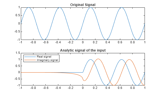
Compute the analytic signal of a sinusoidal input.
t = (-1:0.01:1)'; x = sin(4pit); anaSig = dsp.AnalyticSignal(200); y = anaSig(x);
View the analytic signal.
subplot(2,1,1); plot(t, x) title('Original Signal'); subplot(2,1,2), plot(t, [real(y) imag(y)]); title('Analytic signal of the input') legend('Real signal','Imaginary signal',... 'Location','best');
More About
The analytic signal x = xr +j xi, where the real part xr is the original data and the imaginary part xi contains the Hilbert transform. The imaginary part is a version of the original real sequence with a 90° phase shift. Sines are therefore transformed to cosines, and conversely, cosines are transformed to sines. The Hilbert-transformed series has the same amplitude and frequency content as the original sequence. The transform includes phase information that depends on the phase of the original.
The Hilbert transform is useful in calculating instantaneous attributes of a time series, especially the amplitude and the frequency. The instantaneous amplitude is the amplitude of the complex Hilbert transform. The instantaneous frequency is the time rate of change of the instantaneous phase angle. For a pure sinusoid, the instantaneous amplitude and frequency are constant. The instantaneous phase, however, is a sawtooth, reflecting how the local phase angle varies linearly over a single cycle.
Algorithms
The algorithm computes the Hilbert transform with an equiripple FIR for the specified order n using the Remez exchange algorithm. For higher filter orders, if the equiripple design fails, the algorithm uses a Kaiser window FIR filter instead. In both cases, the filter has a linear phase with a constant group delay of n/2 input samples.
Extended Capabilities
Version History
Introduced in R2012a
When you specify a higher filter order, the dsp.AnalyticSignal object uses the Kaiser window FIR filter to compute the Hilbert transform leading to a robust filter design at higher orders.