Sparse Matrix Operations - MATLAB & Simulink (original) (raw)
Efficiency of Operations
Computational Complexity
The computational complexity of sparse operations is proportional tonnz, the number of nonzero elements in the matrix. Computational complexity also depends linearly on the row size m and column sizen of the matrix, but is independent of the productm*n, the total number of zero and nonzero elements.
The complexity of fairly complicated operations, such as the solution of sparse linear equations, involves factors like ordering and fill-in, which are discussed in the previous section. In general, however, the computer time required for a sparse matrix operation is proportional to the number of arithmetic operations on nonzero quantities.
Algorithmic Details
Sparse matrices propagate through computations according to these rules:
- Functions that accept a matrix and return a scalar or constant-size vector always produce output in full storage format. For example, the size function always returns a full vector, whether its input is full or sparse.
- Functions that accept scalars or vectors and return matrices, such as zeros, ones, rand, and eye, always return full results. This is necessary to avoid introducing sparsity unexpectedly. The sparse analog of
zeros(m,n)is simplysparse(m,n). The sparse analogs ofrandandeyearesprandandspeye, respectively. There is no sparse analog for the functionones. - Unary functions that accept a matrix and return a matrix or vector preserve the storage class of the operand. If
Sis a sparse matrix, thenchol(S)is also a sparse matrix, anddiag(S)is a sparse vector. Columnwise functions such as max and sum also return sparse vectors, even though these vectors can be entirely nonzero. Important exceptions to this rule are thesparseandfullfunctions. - Binary operators yield sparse results if both operands are sparse, and full results if both are full. For mixed operands, the result is full unless the operation preserves sparsity. If
Sis sparse andFis full, thenS+F,S*F, andF\Sare full, whileS.*FandS&Fare sparse. In some cases, the result might be sparse even though the matrix has few zero elements. - Matrix concatenation using either the cat function or square brackets produces sparse results for mixed operands.
Permutations and Reordering
A permutation of the rows and columns of a sparse matrix S can be represented in two ways:
- A permutation matrix
Pacts on the rows ofSasP*Sor on the columns asS*P'. - A permutation vector
p, which is a full vector containing a permutation of1:n, acts on the rows ofSasS(p,:), or on the columns asS(:,p).
For example:
p = [1 3 4 2 5] I = eye(5,5); P = I(p,:) e = ones(4,1); S = diag(11:11:55) + diag(e,1) + diag(e,-1)
p =
1 3 4 2 5P =
 1     0     0     0     0
 0     0     1     0     0
 0     0     0     1     0
 0     1     0     0     0
 0     0     0     0     1
S =
11     1     0     0     0
 1    22     1     0     0
 0     1    33     1     0
 0     0     1    44     1
 0     0     0     1    55
You can now try some permutations using the permutation vector p and the permutation matrix P. For example, the statementsS(p,:) and P*S return the same matrix.
ans =
11     1     0     0     0
 0     1    33     1     0
 0     0     1    44     1
 1    22     1     0     0
 0     0     0     1    55
ans =
11     1     0     0     0
 0     1    33     1     0
 0     0     1    44     1
 1    22     1     0     0
 0     0     0     1    55
Similarly, S(:,p) and S*P' both produce
ans =
11     0     0     1     0
 1     1     0    22     0
 0    33     1     1     0
 0     1    44     0     1
 0     0     1     0    55
If P is a sparse matrix, then both representations use storage proportional to n and you can apply either to S in time proportional to nnz(S). The vector representation is slightly more compact and efficient, so the various sparse matrix permutation routines all return full row vectors with the exception of the pivoting permutation in LU (triangular) factorization, which returns a matrix compatible with the full LU factorization.
To convert between the two permutation representations:
n = 5; I = speye(n); Pr = I(p,:); Pc = I(:,p); pc = (1:n)*Pc
The inverse of P is simply R = P'. You can compute the inverse of p with r(p) = 1:n.
Reordering for Sparsity
Reordering the columns of a matrix can often make its LU or QR factors sparser. Reordering the rows and columns can often make its Cholesky factors sparser. The simplest such reordering is to sort the columns by nonzero count. This is sometimes a good reordering for matrices with very irregular structures, especially if there is great variation in the nonzero counts of rows or columns.
The colperm computes a permutation that orders the columns of a matrix by the number of nonzeros in each column from smallest to largest.
Reordering to Reduce Bandwidth
The reverse Cuthill-McKee ordering is intended to reduce the profile or bandwidth of the matrix. It is not guaranteed to find the smallest possible bandwidth, but it usually does. The symrcm function actually operates on the nonzero structure of the symmetric matrix A + A', but the result is also useful for nonsymmetric matrices. This ordering is useful for matrices that come from one-dimensional problems or problems that are in some sense long and thin.
Approximate Minimum Degree Ordering
The degree of a node in a graph is the number of connections to that node. This is the same as the number of off-diagonal nonzero elements in the corresponding row of the adjacency matrix. The approximate minimum degree algorithm generates an ordering based on how these degrees are altered during Gaussian elimination or Cholesky factorization. It is a complicated and powerful algorithm that usually leads to sparser factors than most other orderings, including column count and reverse Cuthill-McKee. Because keeping track of the degree of each node is very time-consuming, the approximate minimum degree algorithm uses an approximation to the degree, rather than the exact degree.
These MATLAB® functions implement the approximate minimum degree algorithm:
- symamd — Use with symmetric matrices.
- colamd — Use with nonsymmetric matrices and symmetric matrices of the form
A*A'orA'*A.
See Reordering and Factorization of Sparse Matrices for an example usingsymamd.
You can change various parameters associated with details of the algorithms using thespparms function.
For details on the algorithms used by colamd andsymamd, see [5]. The approximate degree the algorithms use is based on [1].
Nested Dissection Ordering
Like the approximate minimum degree ordering, the nested dissection ordering algorithm implemented by the dissect function reorders the matrix rows and columns by considering the matrix to be the adjacency matrix of a graph. The algorithm reduces the problem down to a much smaller scale by collapsing together pairs of vertices in the graph. After reordering the small graph, the algorithm then applies projection and refinement steps to expand the graph back to the original size.
The nested dissection algorithm produces high quality reorderings and performs particularly well with finite element matrices compared to other reordering techniques. For more information about the nested dissection ordering algorithm, see [7].
Factoring Sparse Matrices
LU Factorization
If S is a sparse matrix, the following command returns three sparse matrices L, U, and P such thatP*S = L*U.
lu obtains the factors by Gaussian elimination with partial pivoting. The permutation matrix P has only n nonzero elements. As with dense matrices, the statement [L,U] = lu(S) returns a permuted unit lower triangular matrix and an upper triangular matrix whose product is S. By itself, lu(S) returnsL and U in a single matrix without the pivot information.
The three-output syntax [L,U,P] = lu(S) selectsP via numerical partial pivoting, but does not pivot to improve sparsity in the LU factors. On the other hand, the four-output syntax[L,U,P,Q] = lu(S) selects P via threshold partial pivoting, and selects P and Q to improve sparsity in the LU factors.
You can control pivoting in sparse matrices using
where thresh is a pivot threshold in [0,1]. Pivoting occurs when the diagonal entry in a column has magnitude less than thresh times the magnitude of any sub-diagonal entry in that column. thresh = 0 forces diagonal pivoting. thresh = 1 is the default. (The default for thresh is 0.1 for the four-output syntax).
When you call lu with three or less outputs, MATLAB automatically allocates the memory necessary to hold the sparseL and U factors during the factorization. Except for the four-output syntax, MATLAB does not use any symbolic LU prefactorization to determine the memory requirements and set up the data structures in advance.
Reordering and Factorization of Sparse Matrices
This example shows the effects of reordering and factorization on sparse matrices.
If you obtain a good column permutation p that reduces fill-in, perhaps from symrcm or colamd, then computing lu(S(:,p)) takes less time and storage than computing lu(S).
Create a sparse matrix using the Bucky ball example.
B has exactly three nonzero elements in each row and column.
Create two permutations, r and m using symrcm and symamd respectively.
r = symrcm(B); m = symamd(B);
The two permutations are the symmetric reverse Cuthill-McKee ordering and the symmetric approximate minimum degree ordering.
Create spy plots to show the three adjacency matrices of the Bucky Ball graph with these three different numberings. The local, pentagon-based structure of the original numbering is not evident in the others.
figure subplot(1,3,1) spy(B) title('Original')
subplot(1,3,2) spy(B(r,r)) title('Reverse Cuthill-McKee')
subplot(1,3,3) spy(B(m,m)) title('Min Degree')
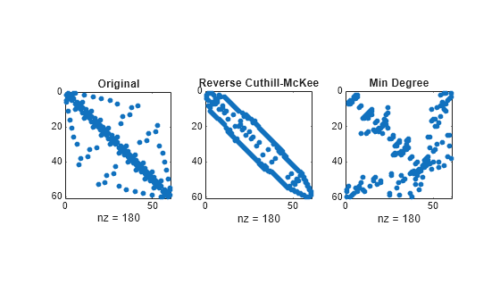
The reverse Cuthill-McKee ordering, r, reduces the bandwidth and concentrates all the nonzero elements near the diagonal. The approximate minimum degree ordering, m, produces a fractal-like structure with large blocks of zeros.
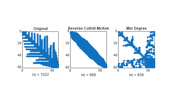
To see the fill-in generated in the LU factorization of the Bucky ball, use speye, the sparse identity matrix, to insert -3s on the diagonal of B.
B = B - 3*speye(size(B));
Since each row sum is now zero, this new B is actually singular, but it is still instructive to compute its LU factorization. When called with only one output argument, lu returns the two triangular factors, L and U, in a single sparse matrix. The number of nonzeros in that matrix is a measure of the time and storage required to solve linear systems involving B.
Here are the nonzero counts for the three permutations being considered.
lu(B)(Original): 1022lu(B(r,r))(Reverse Cuthill-McKee): 968lu(B(m,m))(Approximate minimum degree): 636
Even though this is a small example, the results are typical. The original numbering scheme leads to the most fill-in. The fill-in for the reverse Cuthill-McKee ordering is concentrated within the band, but it is almost as extensive as the first two orderings. For the approximate minimum degree ordering, the relatively large blocks of zeros are preserved during the elimination and the amount of fill-in is significantly less than that generated by the other orderings.
The spy plots below reflect the characteristics of each reordering.
figure subplot(1,3,1) spy(lu(B)) title('Original')
subplot(1,3,2) spy(lu(B(r,r))) title('Reverse Cuthill-McKee')
subplot(1,3,3) spy(lu(B(m,m))) title('Min Degree')
Cholesky Factorization
If S is a symmetric (or Hermitian), positive definite, sparse matrix, the statement below returns a sparse, upper triangular matrix R so that R'*R = S.
chol does not automatically pivot for sparsity, but you can compute approximate minimum degree and profile limiting permutations for use withchol(S(p,p)).
Since the Cholesky algorithm does not use pivoting for sparsity and does not require pivoting for numerical stability, chol does a quick calculation of the amount of memory required and allocates all the memory at the start of the factorization. You can use symbfact, which uses the same algorithm as chol, to calculate how much memory is allocated.
QR Factorization
MATLAB computes the complete QR factorization of a sparse matrixS with
or
but this is often impractical. The unitary matrix Q often fails to have a high proportion of zero elements. A more practical alternative, sometimes known as “the Q-less QR factorization,” is available.
With one sparse input argument and one output argument
returns just the upper triangular portion of the QR factorization. The matrixR provides a Cholesky factorization for the matrix associated with the normal equations:
However, the loss of numerical information inherent in the computation ofS'*S is avoided.
With two input arguments having the same number of rows, and two output arguments, the statement
applies the orthogonal transformations to B, producing C = Q'*B without computing Q.
The Q-less QR factorization allows the solution of sparse least squares problems
with two steps:
If A is sparse, but not square, MATLAB uses these steps for the linear equation solving backslash operator:
Or, you can do the factorization yourself and examine R for rank deficiency.
It is also possible to solve a sequence of least squares linear systems with different right-hand sides, b, that are not necessarily known when R = qr(A) is computed. The approach solves the “semi-normal equationsR'*R*x = A'*b with
and then employs one step of iterative refinement to reduce round off error:
r = b - A*x; e = R(R'(A'*r)); x = x + e
Incomplete Factorizations
The ilu and ichol functions provide approximate, incomplete factorizations, which are useful as preconditioners for sparse iterative methods.
The ilu function produces three incomplete lower-upper (ILU) factorizations: the zero-fill ILU (ILU(0)), a Crout version of ILU (ILUC(tau)), and ILU with threshold dropping and pivoting (ILUTP(tau)). TheILU(0) never pivots and the resulting factors only have nonzeros in positions where the input matrix had nonzeros. Both ILUC(tau) andILUTP(tau), however, do threshold-based dropping with the user-defined drop tolerance tau.
For example:
A = gallery('neumann',1600) + speye(1600); nnz(A)
shows that A has 7840 nonzeros, and its complete LU factorization has 126478 nonzeros. On the other hand, the following code shows the different ILU outputs:
[L,U] = ilu(A); nnz(L)+nnz(U)-size(A,1)
norm(A-(L*U).*spones(A),'fro')./norm(A,'fro')
opts.type = 'ilutp'; opts.droptol = 1e-4; [L,U,P] = ilu(A, opts); nnz(L)+nnz(U)-size(A,1)
norm(PA - LU,'fro')./norm(A,'fro')
opts.type = 'crout'; [L,U,P] = ilu(A, opts); nnz(L)+nnz(U)-size(A,1)
norm(PA-LU,'fro')./norm(A,'fro')
These calculations show that the zero-fill factors have 7840 nonzeros, theILUTP(1e-4) factors have 31147 nonzeros, and theILUC(1e-4) factors have 31083 nonzeros. Also, the relative error of the product of the zero-fill factors is essentially zero on the pattern ofA. Finally, the relative error in the factorizations produced with threshold dropping is on the same order of the drop tolerance, although this is not guaranteed to occur. See the ilu reference page for more options and details.
The ichol function provides zero-fill incomplete Cholesky factorizations (IC(0)) as well as threshold-based dropping incomplete Cholesky factorizations (ICT(tau)) of symmetric, positive definite sparse matrices. These factorizations are the analogs of the incomplete LU factorizations above and have many of the same characteristics. For example:
A = delsq(numgrid('S',200)); nnz(A)
shows that A has 195228 nonzeros, and its complete Cholesky factorization without reordering has 7762589 nonzeros. By contrast:
norm(A-(L*L').*spones(A),'fro')./norm(A,'fro')
opts.type = 'ict'; opts.droptol = 1e-4; L = ichol(A,opts); nnz(L)
norm(A-L*L','fro')./norm(A,'fro')
IC(0) has nonzeros only in the pattern of the lower triangle ofA, and on the pattern of A, the product of the factors matches. Also, the ICT(1e-4) factors are considerably sparser than the complete Cholesky factor, and the relative error between A and L*L' is on the same order of the drop tolerance. It is important to note that unlike the factors provided by chol, the default factors provided by ichol are lower triangular. See the ichol reference page for more information.
Eigenvalues and Singular Values
Two functions are available that compute a few specified eigenvalues or singular values.svds is based on eigs.
Functions to Compute a Few Eigenvalues or Singular Values
| Function | Description |
|---|---|
| eigs | Few eigenvalues |
| svds | Few singular values |
These functions are most frequently used with sparse matrices, but they can be used with full matrices or even with linear operators defined in MATLAB code.
The statement
[V,lambda] = eigs(A,k,sigma)
finds the k eigenvalues and corresponding eigenvectors of the matrixA that are nearest the “shift” sigma. If sigma is omitted, the eigenvalues largest in magnitude are found. Ifsigma is zero, the eigenvalues smallest in magnitude are found. A second matrix, B, can be included for the generalized eigenvalue problem: Aυ = λBυ.
The statement
finds the k largest singular values of A and
[U,S,V] = svds(A,k,'smallest')
finds the k smallest singular values.
The numerical techniques used in eigs and svds are described in [6].
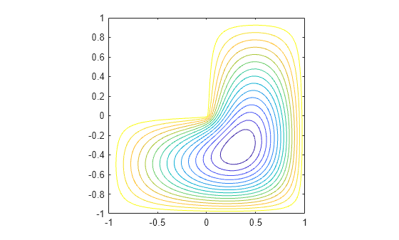
Smallest Eigenvalue of Sparse Matrix
This example shows how to find the smallest eigenvalue and eigenvector of a sparse matrix.
Set up the five-point Laplacian difference operator on a 65-by-65 grid in an _L_-shaped, two-dimensional domain.
L = numgrid('L',65); A = delsq(L);
Determine the order and number of nonzero elements.
A is a matrix of order 2945 with 14,473 nonzero elements.
Compute the smallest eigenvalue and eigenvector.
[v,d] = eigs(A,1,'smallestabs');
Distribute the components of the eigenvector over the appropriate grid points and produce a contour plot of the result.
L(L>0) = full(v(L(L>0))); x = -1:1/32:1; contour(x,x,L,15) axis square
References
[1] Amestoy, P. R., T. A. Davis, and I. S. Duff, “An Approximate Minimum Degree Ordering Algorithm,” SIAM Journal on Matrix Analysis and Applications, Vol. 17, No. 4, Oct. 1996, pp. 886-905.
[2] Barrett, R., M. Berry, T. F. Chan, et al.,Templates for the Solution of Linear Systems: Building Blocks for Iterative Methods, SIAM, Philadelphia, 1994.
[3] Davis, T.A., Gilbert, J. R., Larimore, S.I., Ng, E., Peyton, B., “A Column Approximate Minimum Degree Ordering Algorithm,”Proc. SIAM Conference on Applied Linear Algebra, Oct. 1997, p. 29.
[4] Gilbert, John R., Cleve Moler, and Robert Schreiber, “Sparse Matrices in MATLAB: Design and Implementation,” SIAM J. Matrix Anal. Appl., Vol. 13, No. 1, January 1992, pp. 333-356.
[5] Larimore, S. I., An Approximate Minimum Degree Column Ordering Algorithm, MS Thesis, Dept. of Computer and Information Science and Engineering, University of Florida, Gainesville, FL, 1998.
[6] Saad, Yousef, Iterative Methods for Sparse Linear Equations. PWS Publishing Company, 1996.
[7] Karypis, George and Vipin Kumar. "A Fast and High Quality Multilevel Scheme for Partitioning Irregular Graphs."SIAM Journal on Scientific Computing. Vol. 20, Number 1, 1999, pp. 359–392.