fplot - Plot expression or function - MATLAB (original) (raw)

Plot expression or function

Syntax

Description

fplot([f](#bu6xntj-1-f)) plots the curve defined by the function y = f(x) over the default interval [-5 5] for x.

example

fplot([f](#bu6xntj-1-f),[xinterval](#bu6xntj-1-xinterval)) plots over the specified interval. Specify the interval as a two-element vector of the form [xmin xmax].

example

fplot([funx](#bu6xntj-1-funx),[funy](#bu6xntj-1-funy)) plots the curve defined by x = funx(t) and y = funy(t) over the default interval [-5 5] for t.

example

fplot([funx](#bu6xntj-1-funx),[funy](#bu6xntj-1-funy),[tinterval](#bu6xntj-1-tinterval)) plots over the specified interval. Specify the interval as a two-element vector of the form [tmin tmax].

fplot(___,[LineSpec](#bu6xntj-1%5Fsep%5Fmw%5F3a76f056-2882-44d7-8e73-c695c0c54ca8)) specifies the line style, marker symbol, and line color. For example, '-r' plots a red line. Use this option after any of the input argument combinations in the previous syntaxes.

fplot(___,[Name,Value](#namevaluepairarguments)) specifies line properties using one or more name-value pair arguments. For example, 'LineWidth',2 specifies a line width of 2 points.

example

fplot([ax](#bu6xntj-1-ax),___) plots into the axes specified byax instead of the current axes (gca). Specify the axes as the first input argument.

[x,y] = fplot(___) returns the abscissas and ordinates for the function without creating a plot. This syntax will be removed in a future release. Use the XData and YData properties of the line object, fp, instead.

Note

fplot no longer supports input arguments for specifying the error tolerance or the number of evaluation points. To specify the number of evaluation points, use the MeshDensity property.

Examples

collapse all

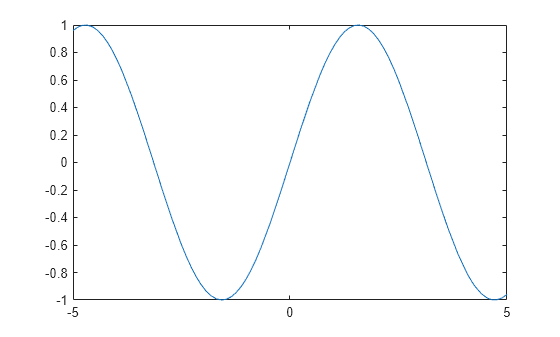
Plot Expression

Plot sin(x) over the default x interval [-5 5].

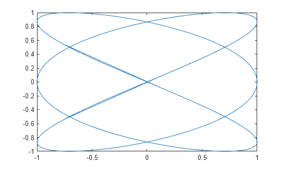
Figure contains an axes object. The axes object contains an object of type functionline.

Plot Parametric Curve

Plot the parametric curve x=cos(3t) and y=sin(2t).

xt = @(t) cos(3t); yt = @(t) sin(2t); fplot(xt,yt)

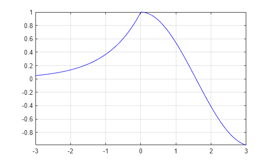
Figure contains an axes object. The axes object contains an object of type parameterizedfunctionline.

Specify Plotting Interval and Plot Piecewise Functions

Plot the piecewise function

ex-3<x<0cos(x)0<x<3.

Plot multiple lines using hold on. Specify the plotting intervals using the second input argument of fplot. Specify the color of the plotted lines as blue using 'b'. When you plot multiple lines in the same axes, the axis limits adjust to incorporate all the data.

fplot(@(x) exp(x),[-3 0],'b') hold on fplot(@(x) cos(x),[0 3],'b') hold off grid on

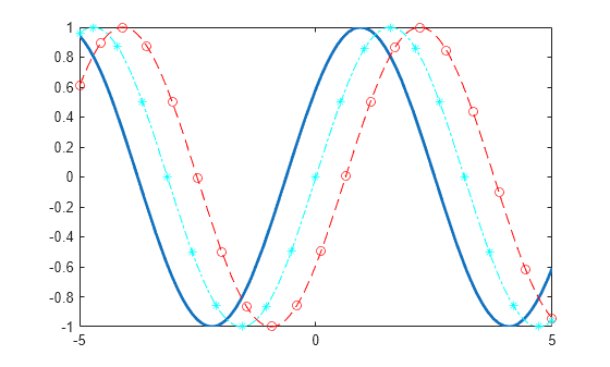
Figure contains an axes object. The axes object contains 2 objects of type functionline.

Specify Line Properties and Display Markers

Plot three sine waves with different phases. For the first, use a line width of 2 points. For the second, specify a dashed red line style with circle markers. For the third, specify a cyan, dash-dotted line style with asterisk markers.

fplot(@(x) sin(x+pi/5),'Linewidth',2); hold on fplot(@(x) sin(x-pi/5),'--or'); fplot(@(x) sin(x),'-.*c') hold off

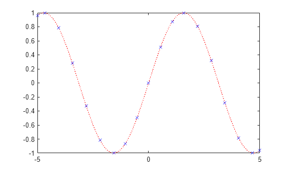
Figure contains an axes object. The axes object contains 3 objects of type functionline.

Modify Line Properties After Creation

Plot sin(x) and assign the function line object to a variable.

Figure contains an axes object. The axes object contains an object of type functionline.

fp = FunctionLine with properties:

 Function: @(x)sin(x)
    Color: [0 0.4470 0.7410]
LineStyle: '-'
LineWidth: 0.5000

Use GET to show all properties

Change the line to a dotted red line by using dot notation to set properties. Add cross markers and set the marker color to blue.

fp.LineStyle = ':'; fp.Color = 'r'; fp.Marker = 'x'; fp.MarkerEdgeColor = 'b';

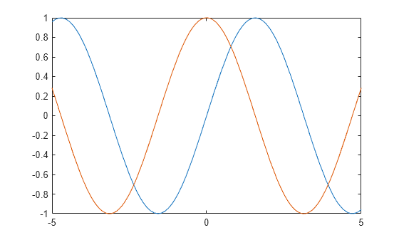
Figure contains an axes object. The axes object contains an object of type functionline.

Plot Multiple Lines in Same Axes

Plot two lines using hold on.

fplot(@(x) sin(x)) hold on fplot(@(x) cos(x)) hold off

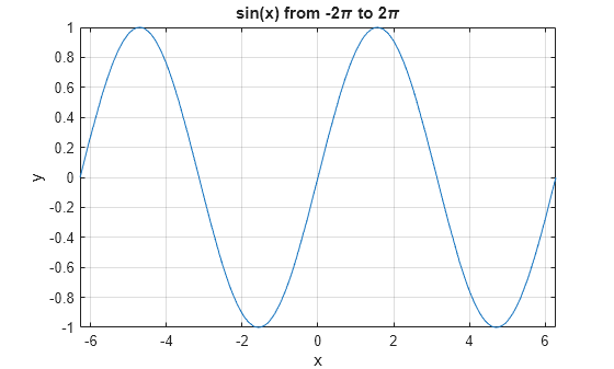
Figure contains an axes object. The axes object contains 2 objects of type functionline.

Add Title and Axis Labels and Format Ticks

Plot sin(x) from -2π to 2π using a function handle. Display the grid lines. Then, add a title and label the _x_-axis and _y_-axis.

fplot(@sin,[-2pi 2pi]) grid on title('sin(x) from -2\pi to 2\pi') xlabel('x'); ylabel('y');

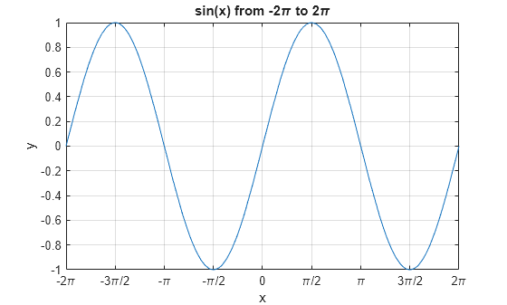
Figure contains an axes object. The axes object with title sin(x) blank from blank - 2 pi blank to blank 2 pi, xlabel x, ylabel y contains an object of type functionline.

Use gca to access the current axes object. Display tick marks along the _x_-axis at intervals of π/2. Format the _x_-axis tick values by setting the XTick and XTickLabel properties of the axes object. Similar properties exist for the _y_-axis.

ax = gca; ax.XTick = -2pi:pi/2:2pi; ax.XTickLabel = {'-2\pi','-3\pi/2','-\pi','-\pi/2','0',... '\pi/2','\pi','3\pi/2','2\pi'};

Figure contains an axes object. The axes object with title sin(x) blank from blank - 2 pi blank to blank 2 pi, xlabel x, ylabel y contains an object of type functionline.

Input Arguments

collapse all

`f` — Function to plot

function handle

Function to plot, specified as a function handle to a named or anonymous function.

Specify a function of the form y = f(x). The function must accept a vector input argument and return a vector output argument of the same size. Use array operators instead of matrix operators for the best performance. For example, use .* (times) instead of * (mtimes).

Note

Support for character vector inputs will be removed in a future release. Use function handles instead.

Example: fplot(@(x) sin(x)) plots sin(x) over the default interval, [-5, 5].

`xinterval` — Interval for `x`

[–5 5] (default) | two-element vector of form [xmin xmax]

Interval for x, specified as a two-element vector of the form [xmin xmax].

`funx` — Parametric function for x coordinates

function handle

Parametric function for x coordinates, specified as a function handle to a named or anonymous function.

Specify a function of the form x = funx(t). The function must accept a vector input argument and return a vector output argument of the same size. Use array operators instead of matrix operators for the best performance. For example, use .* (times) instead of * (mtimes).

Example: funx = @(t) sin(2*t);

`funy` — Parametric function for y coordinates

anonymous function | function handle

Parametric function for y coordinates, specified as a function handle to a named or anonymous function.

Specify a function of the form y = funy(t). The function must accept a vector input argument and return a vector output argument of the same size. Use array operators instead of matrix operators for the best performance. For example, use .* (times) instead of * (mtimes).

Example: funy = @(t) cos(3*t);

`tinterval` — Interval for `t`

[-5 5] (default) | two-element vector of form [tmin tmax]

Interval for t, specified as a two-element vector of the form [tmin tmax].

`ax` — Axes object

axes object

Axes object. If you do not specify an axes object, then fplot uses the current axes (gca).

`LineSpec` — Line style, marker, and color

string scalar | character vector

Line style, marker, and color, specified as a string scalar or character vector containing symbols. The symbols can appear in any order. You do not need to specify all three characteristics (line style, marker, and color). For example, if you omit the line style and specify the marker, then the plot shows only the marker and no line.

Example: "--or" is a red dashed line with circle markers.

Line Style	Description	Resulting Line
"-"	Solid line
"--"	Dashed line
":"	Dotted line
"-."	Dash-dotted line

Marker	Description	Resulting Marker
"o"	Circle
"+"	Plus sign
"*"	Asterisk
"."	Point
"x"	Cross
"_"	Horizontal line
"\|"	Vertical line
"square"	Square
"diamond"	Diamond
"^"	Upward-pointing triangle
"v"	Downward-pointing triangle
">"	Right-pointing triangle
"<"	Left-pointing triangle
"pentagram"	Pentagram
"hexagram"	Hexagram

Color Name	Short Name	RGB Triplet
"red"	"r"	[1 0 0]
"green"	"g"	[0 1 0]
"blue"	"b"	[0 0 1]
"cyan"	"c"	[0 1 1]
"magenta"	"m"	[1 0 1]
"yellow"	"y"	[1 1 0]
"black"	"k"	[0 0 0]
"white"	"w"	[1 1 1]

Name-Value Arguments

Specify optional pairs of arguments asName1=Value1,...,NameN=ValueN, where Name is the argument name and Value is the corresponding value. Name-value arguments must appear after other arguments, but the order of the pairs does not matter.

Before R2021a, use commas to separate each name and value, and enclose Name in quotes.

Example: 'Marker','o','MarkerFaceColor','red'

The properties listed here are only a subset. For a complete list, see FunctionLine Properties or ParameterizedFunctionLine Properties.

Number of evaluation points, specified as a number. The default is 23. Because fplot uses adaptive evaluation, the actual number of evaluation points is greater.

Line color, specified as an RGB triplet, a hexadecimal color code, a color name, or a short name.

For a custom color, specify an RGB triplet or a hexadecimal color code.

An RGB triplet is a three-element row vector whose elements specify the intensities of the red, green, and blue components of the color. The intensities must be in the range [0,1], for example, [0.4 0.6 0.7].
A hexadecimal color code is a string scalar or character vector that starts with a hash symbol (#) followed by three or six hexadecimal digits, which can range from 0 to F. The values are not case sensitive. Therefore, the color codes"#FF8800","#ff8800","#F80", and"#f80" are equivalent.

Alternatively, you can specify some common colors by name. This table lists the named color options, the equivalent RGB triplets, and hexadecimal color codes.

Color Name	Short Name	RGB Triplet	Hexadecimal Color Code
"red"	"r"	[1 0 0]	"#FF0000"
"green"	"g"	[0 1 0]	"#00FF00"
"blue"	"b"	[0 0 1]	"#0000FF"
"cyan"	"c"	[0 1 1]	"#00FFFF"
"magenta"	"m"	[1 0 1]	"#FF00FF"
"yellow"	"y"	[1 1 0]	"#FFFF00"
"black"	"k"	[0 0 0]	"#000000"
"white"	"w"	[1 1 1]	"#FFFFFF"

Here are the RGB triplets and hexadecimal color codes for the default colors MATLAB® uses in many types of plots.

RGB Triplet	Hexadecimal Color Code	Appearance
[0 0.4470 0.7410]	"#0072BD"
[0.8500 0.3250 0.0980]	"#D95319"
[0.9290 0.6940 0.1250]	"#EDB120"
[0.4940 0.1840 0.5560]	"#7E2F8E"
[0.4660 0.6740 0.1880]	"#77AC30"
[0.3010 0.7450 0.9330]	"#4DBEEE"
[0.6350 0.0780 0.1840]	"#A2142F"

Example: "blue"

Example: [0 0 1]

Example: "#0000FF"

Line style, specified as one of the options listed in this table.

Line Style	Description	Resulting Line
"-"	Solid line
"--"	Dashed line
":"	Dotted line
"-."	Dash-dotted line
"none"	No line	No line

Line width, specified as a positive value in points, where 1 point = 1/72 of an inch. If the line has markers, then the line width also affects the marker edges.

The line width cannot be thinner than the width of a pixel. If you set the line width to a value that is less than the width of a pixel on your system, the line displays as one pixel wide.

Marker symbol, specified as one of the values listed in this table. By default, the object does not display markers. Specifying a marker symbol adds markers at each data point or vertex.

Marker	Description	Resulting Marker
"o"	Circle
"+"	Plus sign
"*"	Asterisk
"."	Point
"x"	Cross
"_"	Horizontal line
"\|"	Vertical line
"square"	Square
"diamond"	Diamond
"^"	Upward-pointing triangle
"v"	Downward-pointing triangle
">"	Right-pointing triangle
"<"	Left-pointing triangle
"pentagram"	Pentagram
"hexagram"	Hexagram
"none"	No markers	Not applicable

Marker outline color, specified as "auto", an RGB triplet, a hexadecimal color code, a color name, or a short name. The default value of"auto" uses the same color as the Color property.

For a custom color, specify an RGB triplet or a hexadecimal color code.

An RGB triplet is a three-element row vector whose elements specify the intensities of the red, green, and blue components of the color. The intensities must be in the range [0,1], for example, [0.4 0.6 0.7].
A hexadecimal color code is a string scalar or character vector that starts with a hash symbol (#) followed by three or six hexadecimal digits, which can range from 0 to F. The values are not case sensitive. Therefore, the color codes"#FF8800","#ff8800","#F80", and"#f80" are equivalent.

Alternatively, you can specify some common colors by name. This table lists the named color options, the equivalent RGB triplets, and hexadecimal color codes.

Color Name	Short Name	RGB Triplet	Hexadecimal Color Code	Appearance
"red"	"r"	[1 0 0]	"#FF0000"
"green"	"g"	[0 1 0]	"#00FF00"
"blue"	"b"	[0 0 1]	"#0000FF"
"cyan"	"c"	[0 1 1]	"#00FFFF"
"magenta"	"m"	[1 0 1]	"#FF00FF"
"yellow"	"y"	[1 1 0]	"#FFFF00"
"black"	"k"	[0 0 0]	"#000000"
"white"	"w"	[1 1 1]	"#FFFFFF"
"none"	Not applicable	Not applicable	Not applicable	No color

Here are the RGB triplets and hexadecimal color codes for the default colors MATLAB uses in many types of plots.

RGB Triplet	Hexadecimal Color Code	Appearance
[0 0.4470 0.7410]	"#0072BD"
[0.8500 0.3250 0.0980]	"#D95319"
[0.9290 0.6940 0.1250]	"#EDB120"
[0.4940 0.1840 0.5560]	"#7E2F8E"
[0.4660 0.6740 0.1880]	"#77AC30"
[0.3010 0.7450 0.9330]	"#4DBEEE"
[0.6350 0.0780 0.1840]	"#A2142F"

Marker fill color, specified as "auto", an RGB triplet, a hexadecimal color code, a color name, or a short name. The "auto" value uses the same color as the MarkerEdgeColor property.

For a custom color, specify an RGB triplet or a hexadecimal color code.

An RGB triplet is a three-element row vector whose elements specify the intensities of the red, green, and blue components of the color. The intensities must be in the range [0,1], for example, [0.4 0.6 0.7].
A hexadecimal color code is a string scalar or character vector that starts with a hash symbol (#) followed by three or six hexadecimal digits, which can range from 0 to F. The values are not case sensitive. Therefore, the color codes"#FF8800","#ff8800","#F80", and"#f80" are equivalent.

Alternatively, you can specify some common colors by name. This table lists the named color options, the equivalent RGB triplets, and hexadecimal color codes.

Color Name	Short Name	RGB Triplet	Hexadecimal Color Code	Appearance
"red"	"r"	[1 0 0]	"#FF0000"
"green"	"g"	[0 1 0]	"#00FF00"
"blue"	"b"	[0 0 1]	"#0000FF"
"cyan"	"c"	[0 1 1]	"#00FFFF"
"magenta"	"m"	[1 0 1]	"#FF00FF"
"yellow"	"y"	[1 1 0]	"#FFFF00"
"black"	"k"	[0 0 0]	"#000000"
"white"	"w"	[1 1 1]	"#FFFFFF"
"none"	Not applicable	Not applicable	Not applicable	No color

Here are the RGB triplets and hexadecimal color codes for the default colors MATLAB uses in many types of plots.

RGB Triplet	Hexadecimal Color Code	Appearance
[0 0.4470 0.7410]	"#0072BD"
[0.8500 0.3250 0.0980]	"#D95319"
[0.9290 0.6940 0.1250]	"#EDB120"
[0.4940 0.1840 0.5560]	"#7E2F8E"
[0.4660 0.6740 0.1880]	"#77AC30"
[0.3010 0.7450 0.9330]	"#4DBEEE"
[0.6350 0.0780 0.1840]	"#A2142F"

Example: [0.3 0.2 0.1]

Example: "green"

Example: "#D2F9A7"

Marker size, specified as a positive value in points, where 1 point = 1/72 of an inch.

Output Arguments

collapse all

`fp` — One or more `FunctionLine` or `ParameterizedFunctionLine` objects

scalar | vector

One or more FunctionLine or ParameterizedFunctionLine objects, returned as a scalar or a vector.

If you use the fplot(f) syntax or a variation of this syntax, then fplot returns FunctionLine objects.
If you use the fplot(funx,funy) syntax or a variation of this syntax, then fplot returns ParameterizedFunctionLine objects.

You can use these objects to query and modify properties of a specific line. For a list of properties, see FunctionLine Properties and ParameterizedFunctionLine Properties.

Tips

Use element-wise operators for the best performance and to avoid a warning message. For example, use x.*y instead of x*y. For more information, see Array vs. Matrix Operations.
When you zoom in on the chart, fplot replots the data, which can reveal hidden details.

Extended Capabilities

GPU Arrays

Accelerate code by running on a graphics processing unit (GPU) using Parallel Computing Toolbox™.

The fplot function supports GPU array input with these usage notes and limitations:

This function accepts GPU arrays, but does not run on a GPU.

For more information, see Run MATLAB Functions on a GPU (Parallel Computing Toolbox).

Distributed Arrays

Partition large arrays across the combined memory of your cluster using Parallel Computing Toolbox™.

Usage notes and limitations:

This function operates on distributed arrays, but executes in the client MATLAB.

For more information, see Run MATLAB Functions with Distributed Arrays (Parallel Computing Toolbox).

Version History

Introduced before R2006a

fplot - Plot expression or function - MATLAB (original) (raw)

Syntax

Description

Examples

Plot Expression

Plot Parametric Curve

Specify Plotting Interval and Plot Piecewise Functions

Specify Line Properties and Display Markers

Modify Line Properties After Creation

Plot Multiple Lines in Same Axes

Add Title and Axis Labels and Format Ticks

Input Arguments

f — Function to plot

xinterval — Interval for x

funx — Parametric function for x coordinates

funy — Parametric function for y coordinates

tinterval — Interval for t

ax — Axes object

LineSpec — Line style, marker, and color

Name-Value Arguments

Output Arguments

fp — One or more FunctionLine or ParameterizedFunctionLine objects

Tips

Extended Capabilities

GPU Arrays

Distributed Arrays

Version History

`f` — Function to plot

`xinterval` — Interval for `x`

`funx` — Parametric function for x coordinates

`funy` — Parametric function for y coordinates

`tinterval` — Interval for `t`

`ax` — Axes object

`LineSpec` — Line style, marker, and color

`fp` — One or more `FunctionLine` or `ParameterizedFunctionLine` objects