Bayesian Optimization Plot Functions - MATLAB & Simulink (original) (raw)
Built-In Plot Functions
There are two sets of built-in plot functions.
| Model Plots — Apply When D ≤ 2 | Description |
|---|---|
| @plotAcquisitionFunction | Plot the acquisition function surface. |
| @plotConstraintModels | Plot each constraint model surface. Negative values indicate feasible points.Also plot a_P_(feasible) surface.Also plot the error model, if it exists, which ranges from –1 to 1. Negative values mean that the model probably does not error, positive values mean that it probably does error. The model is:Plotted error = 2*Probability(error) – 1. |
| @plotObjectiveEvaluationTimeModel | Plot the objective function evaluation time model surface. |
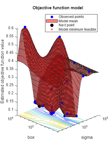
| @plotObjectiveModel | Plot the fun model surface, the estimated location of the minimum, and the location of the next proposed point to evaluate. For one-dimensional problems, plot envelopes one credible interval above and below the mean function, and envelopes one noise standard deviation above and below the mean. |
| Trace Plots — Apply to All D | Description |
|---|---|
| @plotObjective | Plot each observed function value versus the number of function evaluations. |
| @plotObjectiveEvaluationTime | Plot each observed function evaluation run time versus the number of function evaluations. |
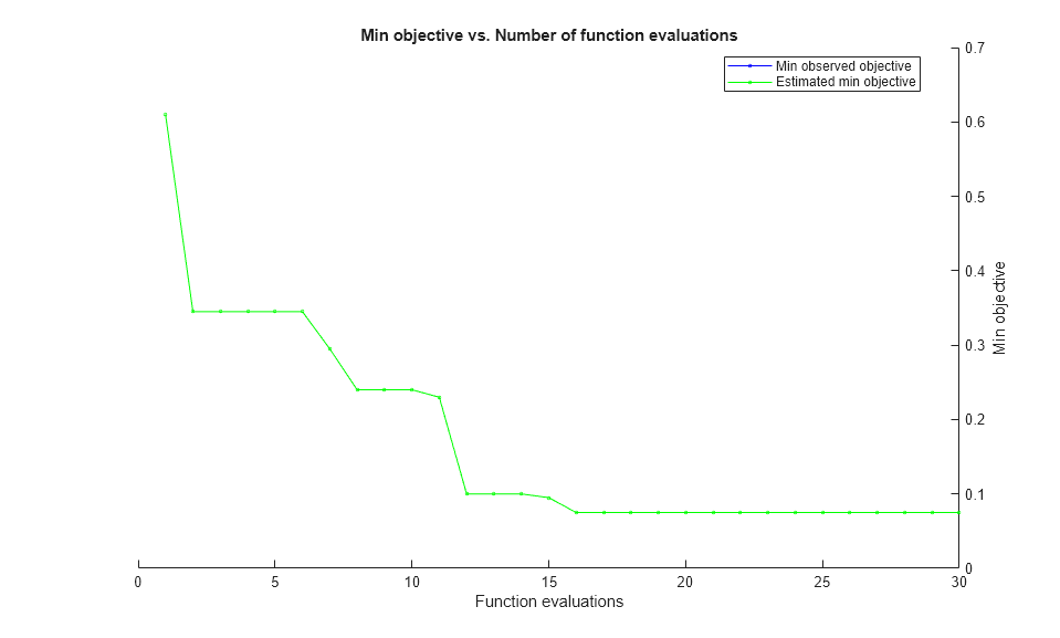
| @plotMinObjective | Plot the minimum observed and estimated function values versus the number of function evaluations. |
| @plotElapsedTime | Plot three curves: the total elapsed time of the optimization, the total function evaluation time, and the total modeling and point selection time, all versus the number of function evaluations. |
Note
When there are coupled constraints, iterative display and plot functions can give counterintuitive results such as:
- A minimum objective plot can increase.
- The optimization can declare a problem infeasible even when it showed an earlier feasible point.
The reason for this behavior is that the decision about whether a point is feasible can change as the optimization progresses. bayesopt determines feasibility with respect to its constraint model, and this model changes as bayesopt evaluates points. So a “minimum objective” plot can increase when the minimal point is later deemed infeasible, and the iterative display can show a feasible point that is later deemed infeasible.
Custom Plot Function Syntax
A custom plot function has the same syntax as a custom output function (see Bayesian Optimization Output Functions):
stop = plotfun(results,state)
bayesopt passes the results and state variables to your function. Your function returns stop, which you set to true to halt the iterations, or to false to continue the iterations.
results is an object of class BayesianOptimization that contains the available information on the computations.
state has these possible values:
'initial'—bayesoptis about to start iterating. Use this state to set up a plot or to perform other initializations.'iteration'—bayesoptjust finished an iteration. Generally, you perform most of the plotting or other calculations in this state.'done'—bayesoptjust finished its final iteration. Clean up plots or otherwise prepare for the plot function to shut down.
Create a Custom Plot Function
This example shows how to create a custom plot function for bayesopt. It further shows how to use information in the UserData property of a BayesianOptimization object.
Problem Statement
The problem is to find parameters of a Support Vector Machine (SVM) classification to minimize the cross-validated loss. The specific model is the same as in Optimize Cross-Validated Classifier Using bayesopt. Therefore, the objective function is essentially the same, except it also computes UserData, in this case the number of support vectors in an SVM model fitted to the current parameters.
Create a custom plot function that plots the number of support vectors in the SVM model as the optimization progresses. To give the plot function access to the number of support vectors, create a third output, UserData, to return the number of support vectors.
Objective Function
Create an objective function that computes the cross-validation loss for a fixed cross-validation partition, and that returns the number of support vectors in the resulting model.
function [f,viol,nsupp] = mysvmminfn(x,cdata,grp,c) SVMModel = fitcsvm(cdata,grp,'KernelFunction','rbf',... 'KernelScale',x.sigma,'BoxConstraint',x.box); f = kfoldLoss(crossval(SVMModel,'CVPartition',c)); viol = []; nsupp = sum(SVMModel.IsSupportVector); end
Custom Plot Function
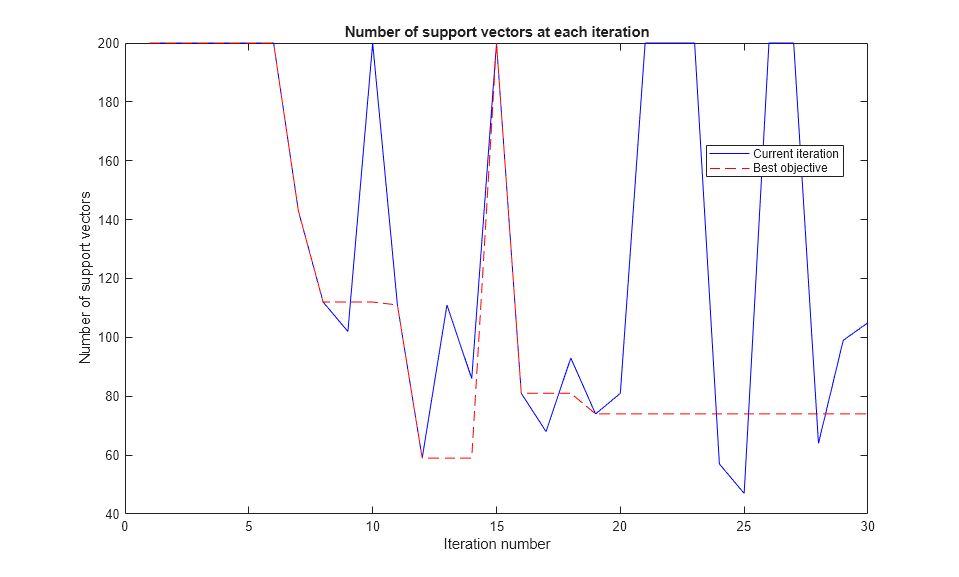
Create a custom plot function that uses the information computed in UserData. Have the function plot both the current number of constraints and the number of constraints for the model with the best objective function found.
function stop = svmsuppvec(results,state) persistent hs nbest besthist nsupptrace stop = false; switch state case 'initial' hs = figure; besthist = []; nbest = 0; nsupptrace = []; case 'iteration' figure(hs) nsupp = results.UserDataTrace{end}; % get nsupp from UserDataTrace property. nsupptrace(end+1) = nsupp; % accumulate nsupp values in a vector. if (results.ObjectiveTrace(end) == min(results.ObjectiveTrace)) || (length(results.ObjectiveTrace) == 1) % current is best nbest = nsupp; end besthist = [besthist,nbest]; plot(1:length(nsupptrace),nsupptrace,'b',1:length(besthist),besthist,'r--') xlabel 'Iteration number' ylabel 'Number of support vectors' title 'Number of support vectors at each iteration' legend('Current iteration','Best objective','Location','best') drawnow end
Set Up the Model
Generate ten base points for each class.
rng default grnpop = mvnrnd([1,0],eye(2),10); redpop = mvnrnd([0,1],eye(2),10);
Generate 100 data points of each class.
redpts = zeros(100,2);grnpts = redpts; for i = 1:100 grnpts(i,:) = mvnrnd(grnpop(randi(10),:),eye(2)*0.02); redpts(i,:) = mvnrnd(redpop(randi(10),:),eye(2)*0.02); end
Put the data into one matrix, and make a vector grp that labels the class of each point.
cdata = [grnpts;redpts]; grp = ones(200,1); % Green label 1, red label -1 grp(101:200) = -1;
Check the basic classification of all the data using the default SVM parameters.
SVMModel = fitcsvm(cdata,grp,'KernelFunction','rbf','ClassNames',[-1 1]);
Set up a partition to fix the cross validation. Without this step, the cross validation is random, so the objective function is not deterministic.
c = cvpartition(200,'KFold',10);
Check the cross-validation accuracy of the original fitted model.
loss = kfoldLoss(fitcsvm(cdata,grp,'CVPartition',c,... 'KernelFunction','rbf','BoxConstraint',SVMModel.BoxConstraints(1),... 'KernelScale',SVMModel.KernelParameters.Scale))
Prepare Variables for Optimization
The objective function takes an input z = [rbf_sigma,boxconstraint] and returns the cross-validation loss value of z. Take the components of z as positive, log-transformed variables between 1e-5 and 1e5. Choose a wide range because you do not know which values are likely to be good.
sigma = optimizableVariable('sigma',[1e-5,1e5],'Transform','log'); box = optimizableVariable('box',[1e-5,1e5],'Transform','log');
Set Plot Function and Call the Optimizer
Search for the best parameters [sigma,box] using bayesopt. For reproducibility, choose the 'expected-improvement-plus' acquisition function. The default acquisition function depends on run time, so it can give varying results.
Plot the number of support vectors as a function of the iteration number, and plot the number of support vectors for the best parameters found.
obj = @(x)mysvmminfn(x,cdata,grp,c); results = bayesopt(obj,[sigma,box],... 'IsObjectiveDeterministic',true,'Verbose',0,... 'AcquisitionFunctionName','expected-improvement-plus',... 'PlotFcn',{@svmsuppvec,@plotObjectiveModel,@plotMinObjective})
results =
BayesianOptimization with properties:
                  ObjectiveFcn: @(x)mysvmminfn(x,cdata,grp,c)
          VariableDescriptions: [1x2 optimizableVariable]
                       Options: [1x1 struct]
                  MinObjective: 0.0750
               XAtMinObjective: [1x2 table]
         MinEstimatedObjective: 0.0750
      XAtMinEstimatedObjective: [1x2 table]
       NumObjectiveEvaluations: 30
              TotalElapsedTime: 53.9146
                     NextPoint: [1x2 table]
                        XTrace: [30x2 table]
                ObjectiveTrace: [30x1 double]
              ConstraintsTrace: []
                 UserDataTrace: {30x1 cell}
  ObjectiveEvaluationTimeTrace: [30x1 double]
            IterationTimeTrace: [30x1 double]
                    ErrorTrace: [30x1 double]
              FeasibilityTrace: [30x1 logical]
   FeasibilityProbabilityTrace: [30x1 double]
           IndexOfMinimumTrace: [30x1 double]
         ObjectiveMinimumTrace: [30x1 double]
EstimatedObjectiveMinimumTrace: [30x1 double]