Bayesian Optimization Output Functions - MATLAB & Simulink (original) (raw)
What Is a Bayesian Optimization Output Function?
An output function is a function that is called at the end of every iteration of bayesopt. An output function can halt iterations. It can also create plots, save information to your workspace or to a file, or perform any other calculation you like.
Other than halting the iterations, output functions cannot change the course of a Bayesian optimization. They simply monitor the progress of the optimization.
Built-In Output Functions
These built-in output functions save your optimization results to a file or to the workspace.
@assignInBase— Saves your results after each iteration to a variable named'BayesoptResults'in your workspace. To choose a different name, pass theSaveVariableNamename-value argument.@saveToFile— Saves your results after each iteration to a file named'BayesoptResults.mat'in your current folder. To choose a different name or folder, pass theSaveFileNamename-value argument.
For example, to save the results after each iteration to a workspace variable named 'BayesIterations',
results = bayesopt(fun,vars,'OutputFcn',@assignInBase, ... 'SaveVariableName','BayesIterations')
Custom Output Functions
Write a custom output function with signature
stop = outputfun(results,state)
bayesopt passes the results and state variables to your function. Your function returns stop, which you set to true to halt the iterations, or to false to allow the iterations to continue.
results is an object of class BayesianOptimization. results contains the available information on the computations so far.
state has possible values:
'initial'—bayesoptis about to start iterating.'iteration'—bayesoptjust finished an iteration.'done'—bayesoptjust finished its final iteration.
For an example, see Bayesian Optimization Output Function.
Bayesian Optimization Output Function
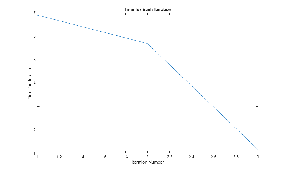
This example shows how to use a custom output function with Bayesian optimization. The output function halts the optimization when the objective function, which is the cross-validation error rate, drops below 13%. The output function also plots the time for each iteration.
function stop = outputfun(results,state) persistent h stop = false; switch state case 'initial' h = figure; case 'iteration' if results.MinObjective < 0.13 stop = true; end figure(h) tms = results.IterationTimeTrace; plot(1:numel(tms),tms') xlabel('Iteration Number') ylabel('Time for Iteration') title('Time for Each Iteration') drawnow end end
The objective function is the cross validation loss of the KNN classification of the ionosphere data. Load the data and, for reproducibility, set the default random stream.
load ionosphere rng default
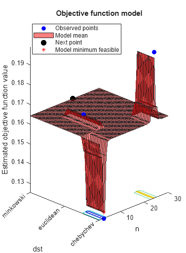
Optimize over neighborhood size from 1 through 30, and for three distance metrics.
num = optimizableVariable('n',[1,30],'Type','integer'); dst = optimizableVariable('dst',{'chebychev','euclidean','minkowski'},'Type','categorical'); vars = [num,dst];
Set the cross-validation partition and objective function. For reproducibility, set the AcquisitionFunctionName to 'expected-improvement-plus'. Run the optimization.
c = cvpartition(351,'Kfold',5); fun = @(x)kfoldLoss(fitcknn(X,Y,'CVPartition',c,'NumNeighbors',x.n,... 'Distance',char(x.dst),'NSMethod','exhaustive')); results = bayesopt(fun,vars,'OutputFcn',@outputfun,... 'AcquisitionFunctionName','expected-improvement-plus');
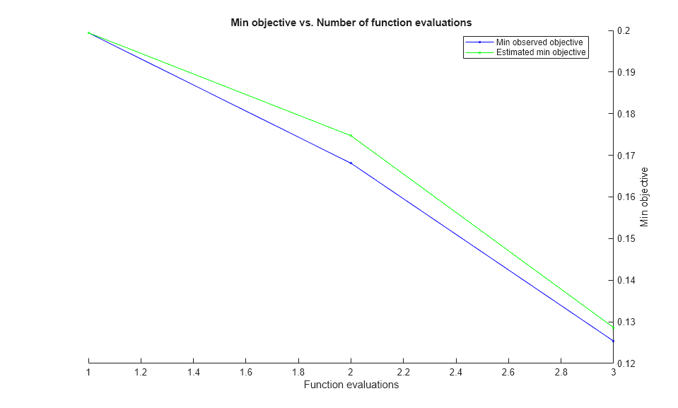
|=====================================================================================================| | Iter | Eval | Objective | Objective | BestSoFar | BestSoFar | n | dst | | | result | | runtime | (observed) | (estim.) | | | |=====================================================================================================| | 1 | Best | 0.19943 | 0.38956 | 0.19943 | 0.19943 | 24 | chebychev | | 2 | Best | 0.16809 | 0.26602 | 0.16809 | 0.1747 | 9 | euclidean | | 3 | Best | 0.12536 | 0.17037 | 0.12536 | 0.12861 | 3 | chebychev |
Optimization completed. Total function evaluations: 3 Total elapsed time: 6.8948 seconds Total objective function evaluation time: 0.82595
Best observed feasible point:
n dst
_ _________
3 chebychevObserved objective function value = 0.12536 Estimated objective function value = 0.12861 Function evaluation time = 0.17037
Best estimated feasible point (according to models):
n dst
_ _________
3 chebychevEstimated objective function value = 0.12861 Estimated function evaluation time = 0.26023