Compare Custom Solvers Using Custom Training Loop - MATLAB & Simulink (original) (raw)

This example shows how to train a deep learning network with different custom solvers and compare their accuracies.

In a deep learning network, a solver refers to an optimization algorithm used to minimize the loss function of the network during training. The choice of solver can affect the speed of convergence and the accuracy of the final model. Some solvers may converge faster, while others might be more stable or require less fine-tuning of hyperparameters.

For most tasks, you can train a neural network using the trainnet and trainingOptions function and specifying a built-in solver like Adam or SGDM. For an example showing how to train a neural network using the trainnet function, see Create Simple Deep Learning Neural Network for Classification.

If you want to use a different solver to improve the accuracy or convergence rate of a network, you can define a custom solver and use a custom training loop.

This example trains a network using three different solvers not provided by the trainingOptions function:

1. AdamW – Adam with decoupled weight decay. This solver decouples the weight decay from the optimization step taken with respect to the loss function and improves Adam's generalization performance. [1]
2. AMSGrad – Adam with a stable gradient. This solver introduces a "long-term memory" of past gradients to fix issues of Adam where it fails to converge to an optimal solution. [2]
3. LAMB – Layer-wise adaptive moments for batch training. This solver adapts the learning rate on a per-layer basis to reduce training time for large batch sizes while maintaining the generalization performance of Adam. [3]

Load Training Data

Load the digits data as an image datastore using the imageDatastore function and specify the folder containing the image data.

unzip("DigitsData.zip")

imds = imageDatastore("DigitsData", ... IncludeSubfolders=true, ... LabelSource="foldernames");

Partition the data into training, validation, and test sets. Set aside 10% of the data for validation and 10% of the data for testing using the splitEachLabel function.

[imdsTrain,imdsValidation,imdsTest] = splitEachLabel(imds,0.8,0.1,"randomize");

The network used in this example requires input images of size 28-by-28-by-1. To automatically resize the training images, use an augmented image datastore. Specify additional augmentation operations to perform on the training images: randomly translate the images up to 5 pixels in the horizontal and vertical axes. Data augmentation helps prevent the network from overfitting and memorizing the exact details of the training images.

inputSize = [28 28 1]; pixelRange = [-5 5];

imageAugmenter = imageDataAugmenter( ... RandXTranslation=pixelRange, ... RandYTranslation=pixelRange);

augimdsTrain = augmentedImageDatastore(inputSize(1:2),imdsTrain,DataAugmentation=imageAugmenter);

To automatically resize the validation and testing images without performing further data augmentation, use an augmented image datastore without specifying any additional preprocessing operations.

augimdsValidation = augmentedImageDatastore(inputSize(1:2),imdsValidation); augimdsTest = augmentedImageDatastore(inputSize(1:2),imdsTest);

Determine the number of classes in the training data.

classes = categories(imdsTrain.Labels); numClasses = numel(classes);

Define Network

Define the network for image classification.

• For image input, specify an image input layer with input size matching the training data.
• Do not normalize the image input, set the Normalization option of the input layer to "none".
• Specify three convolution-batchnorm-ReLU blocks.
• For all convolution layers specify 32 filters of size 5.
• For classification, specify a fully connected layer with size matching the number of classes
• To map the output to probabilities, include a softmax layer.

layers = [ imageInputLayer(inputSize, Normalization="none") convolution2dLayer(5, 32) batchNormalizationLayer reluLayer convolution2dLayer(5, 32) batchNormalizationLayer reluLayer convolution2dLayer(5, 32) batchNormalizationLayer reluLayer globalAveragePooling2dLayer fullyConnectedLayer(numClasses) softmaxLayer];

Create a dlnetwork object from the layer array.

net = dlnetwork with properties:

     Layers: [13×1 nnet.cnn.layer.Layer]
Connections: [12×2 table]
 Learnables: [14×3 table]
      State: [6×3 table]
 InputNames: {'imageinput'}
OutputNames: {'softmax'}
Initialized: 1

View summary with summary.

Define Model Loss Function

Training a deep neural network is an optimization task. By considering a neural network as a function , where X is the network input, and θ is the set of learnable parameters, you can optimize θ so that it minimizes some loss value based on the training data. For example, optimize the learnable parameters θ such that for a given inputs X with a corresponding targets T, they minimize the error between the predictions and T.

Define the modelLoss function. The modelLoss function takes a dlnetwork object net, a mini-batch of input data X with corresponding targets T and returns the loss, the gradients of the loss with respect to the learnable parameters in net, and the network state. To compute the gradients automatically, use the dlgradient function.

function [loss,gradients,state] = modelLoss(net,X,T)

% Forward data through network. [Y,state] = forward(net,X);

% Calculate cross-entropy loss. loss = crossentropy(Y,T);

% Calculate gradients of loss with respect to learnable parameters. gradients = dlgradient(loss,net.Learnables);

end

Define Update Functions

Implement solver algorithms and define functions that update the learnables of a deep learning network using these solvers.

Define AdamW Function

The function adamWStep implements the AdamW algorithm. The update step with weights decoupling is given by

Θupdate=σbiasmlvl+ε+λθl

where

• σbias is a bias correction term
• ml is the moving average of parameter gradients
• vl is the moving average of squared parameter gradients
• ε is a small constant that avoids division by 0
• λ is the weight decay coefficient
• θ is the parameter vector.

We then obtain the update function

θl+1=θl-α⋅Θupdate

where α>0 is the learning rate.

The adamwupdate function updates the dlnetwork object using dlupdate.

function [parameters,avgGrad,avgSqGrad] = adamWStep(parameters,avgGrad,avgSqGrad,gradients,... iteration,learnRate,gradDecay,sqGradDecay,... weightDecay,epsilon)

% Update the moving averages of gradients. avgGrad = gradDecay * avgGrad + (1-gradDecay) .* gradients; avgSqGrad = sqGradDecay * avgSqGrad + (1-sqGradDecay) .* (gradients .^ 2);

% Bias correction. biasCorrection = sqrt(1-sqGradDecay^iteration)/(1-gradDecay^iteration);

% Update parameters. updateStep = biasCorrection .* avgGrad ./ (sqrt(avgSqGrad) + epsilon) + weightDecay * parameters; parameters = parameters - learnRate .* updateStep;

end

function [net,avgGrad,avgSqGrad] = adamwupdate(net,avgGrad,avgSqGrad,gradients,... iteration,learnRate,gradDecay,sqGradDecay,... weightDecay,epsilon)

% Create arrays for moving averages of gradients for the first step. if iteration == 1 [avgGrad,avgSqGrad] = initializeSolverParameters(net); end

% Update network using dlupdate. updateFcn = @(net,avgGrad,avgSqGrad,gradients) adamWStep(net,avgGrad,avgSqGrad,gradients,... iteration,learnRate,gradDecay,sqGradDecay,... weightDecay,epsilon);

[net,avgGrad,avgSqGrad] = dlupdate(updateFcn,net,avgGrad,avgSqGrad,gradients);

end

Define AMSGrad Function

The function amsgradStep implements the AMSGrad solver. This solver addresses issues where the Adam solver fail to converge to the optimal solution by storing the maximum of all squares of gradients up till the current time step

vlˆ=max(vl-1ˆ,vl)

The update step is given by

Θupdate=σbiasmlvlˆ+ε

We then obtain the update function

θl+1=θl-α⋅Θupdate

The amsgradupdate function updates the dlnetwork object using dlupdate.

function [parameters,avgGrad,avgSqGrad,avgSqGradMax] = amsgradStep(parameters,avgGrad,avgSqGrad,... avgSqGradMax,gradients,... iteration,learnRate,... gradDecay,sqGradDecay,epsilon)

% Update the moving averages of gradients. avgGrad = gradDecay * avgGrad + (1-gradDecay) .* gradients; avgSqGrad = sqGradDecay * avgSqGrad + (1-sqGradDecay) .* (gradients .^ 2); avgSqGradMax = max(avgSqGradMax,avgSqGrad);

% Bias correction term and the update step. biasCorrection = sqrt(1-sqGradDecay^iteration)/(1-gradDecay^iteration); updateStep = biasCorrection .* avgGrad ./ (sqrt(avgSqGradMax) + epsilon);

% Update parameters. parameters = parameters - learnRate .* updateStep;

end

function [net,avgGrad,avgSqGrad,avgSqGradMax] = amsgradupdate(net,avgGrad,avgSqGrad,... avgSqGradMax,gradients,... iteration,learnRate,... gradDecay,sqGradDecay,epsilon)

% Create arrays for moving averages of gradients for the first step. if iteration ==1 [avgGrad,avgSqGrad,avgSqGradMax] = initializeSolverParameters(net); end

% Update network using dlupdate. updateFcn = @(net,avgGrad,avgSqGrad,avgSqGradMax,gradients) amsgradStep(net,avgGrad,avgSqGrad,... avgSqGradMax,gradients,... iteration,learnRate,... gradDecay,sqGradDecay,epsilon);

[net,avgGrad,avgSqGrad,avgSqGradMax] = dlupdate(updateFcn,net,avgGrad,avgSqGrad,avgSqGradMax,gradients);

end

Define LAMB Function with Weight Decoupling

The function lambStep implements the LAMB solver. It differs from AdamW by adding an extra trust ratio term to achieve a layer-wise adaptive learning rate.

σtrust=‖θl‖‖Θupdate‖

So the update function is given by

θl+1=θl-α⋅σtrust⋅Θupdate

The lambupdate function updates the dlnetwork object using dlupdate.

function [parameters,avgGrad,avgSqGrad] = lambStep(parameters,avgGrad,avgSqGrad,gradients,... iteration,learnRate,gradDecay,sqGradDecay,... weightDecay,epsilon)

% Update the moving averages of gradients. avgGrad = gradDecay * avgGrad + (1-gradDecay) .* gradients; avgSqGrad = sqGradDecay * avgSqGrad + (1-sqGradDecay) .* (gradients .^ 2);

% Bias correction term and the update step. biasCorrection = sqrt(1-sqGradDecay^iteration)/(1-gradDecay^iteration); updateStep = biasCorrection .* avgGrad ./ (sqrt(avgSqGrad) + epsilon) + weightDecay * parameters;

% Calculate the Frobenius norms needed for the trust ratio. weightNorm = sqrt(sum(parameters .^ 2,"all")); updateNorm = sqrt(sum(updateStep .^ 2,"all"));

% Calculate the trust ratio. trustRatio = 1; if weightNorm > 0 && updateNorm > 0 trustRatio = weightNorm / updateNorm; end

% Update parameters parameters = parameters - learnRate .* trustRatio .* updateStep;

end

function [net,avgGrad,avgSqGrad] = lambupdate(net,avgGrad,avgSqGrad,gradients,... iteration,learnRate,gradDecay,sqGradDecay,... weightDecay,epsilon)

% Create arrays for moving averages of gradients for the first step. if iteration == 1 [avgGrad,avgSqGrad] = initializeSolverParameters(net); end

% Update network using dlupdate. updateFcn = @(net,avgGrad,avgSqGrad,gradients) lambStep(net,avgGrad,avgSqGrad,gradients,... iteration,learnRate,gradDecay,sqGradDecay,... weightDecay,epsilon);

[net,avgGrad,avgSqGrad] = dlupdate(updateFcn,net,avgGrad,avgSqGrad,gradients);

end

Solver Parameter Initialization Function

The solvers require moving averages of gradients to update learnable parameters. These moving averages must have sizes that match the parameters of the neural network. The initializeSolverParameters function creates these solver parameters.

function varargout = initializeSolverParameters(net)

parameters = net.Learnables; solverParams = parameters;

for i = 1:size(parameters,1) paramSize = size(parameters.Value{i}); solverParams.Value{i} = zeros(paramSize, 'like', parameters.Value{i}); end

varargout = cell(1,nargout); for i = 1:nargout varargout{i} = solverParams; end

end

Specify Training Options

Train for fifteen epochs with a mini-batch size of 128. Calculate the validation loss and accuracy every 20 iterations.

numEpochs = 15; miniBatchSize = 128; validationFrequency = 20;

Specify the parameters for optimization:

• Specify a learning rate of 0.01.
• Specify a weight decay factor of 0.01 for AdamW and LAMB for weight decoupling.
• Specify a gradient decay factor of 0.9, a squared gradient decay factor of 0.999, and a small constant of 1e-8 for all solvers.

learnRate = 0.01; gradDecay = 0.9; sqGradDecay = 0.999; weightDecay = 0.01; epsilon = 1e-8;

Train Model

Train three deep learning networks with different custom solvers using a custom training loop.

Create a minibatchqueue object that processes and manages mini-batches of images during training. For each mini-batch:

• Use the custom mini-batch preprocessing function preprocessMiniBatch to convert the labels to one-hot encoded variables.
• Format the image data with the dimension labels "SSCB" (spatial, spatial, channel, batch). By default, the minibatchqueue object converts the data to dlarray objects with underlying type single. Do not format the class labels.
• Discard partial mini-batches.
• Train on a GPU if one is available. By default, the minibatchqueue object converts each output to a gpuArray if a GPU is available. Using a GPU requires Parallel Computing Toolbox™ and a supported GPU device. For information on supported devices, see GPU Computing Requirements (Parallel Computing Toolbox).

mbq = minibatchqueue(augimdsTrain,... MiniBatchSize=miniBatchSize,... MiniBatchFcn=@preprocessMiniBatch,... MiniBatchFormat=["SSCB" ""], ... PartialMiniBatch="discard");

Mini Batch Preprocessing Function

The preprocessMiniBatch function preprocesses a mini-batch of predictors and labels using the following steps:

1. Preprocess the images using the preprocessMiniBatchPredictors function.
2. Extract the label data from the incoming cell array and concatenate into a categorical array along the second dimension.
3. One-hot encode the categorical labels into numeric arrays. Encoding into the first dimension produces an encoded array that matches the shape of the network output.

function [X,T] = preprocessMiniBatch(dataX,dataT)

% Preprocess predictors. X = preprocessMiniBatchPredictors(dataX);

% Extract label data from cell and concatenate. T = cat(2,dataT{1:end});

% One-hot encode labels. T = onehotencode(T,1);

end

Mini-Batch Predictors Preprocessing Function

The preprocessMiniBatchPredictors function preprocesses a mini-batch of predictors by extracting the image data from the input cell array and concatenate into a numeric array. For grayscale input, concatenating over the fourth dimension adds a third dimension to each image, to use as a singleton channel dimension.

function X = preprocessMiniBatchPredictors(dataX)

% Concatenate. X = cat(4,dataX{1:end});

end

Calculate the total number of iterations for the training progress monitor.

numObservationsTrain = numel(imdsTrain.Files); numIterationsPerEpoch = floor(numObservationsTrain / miniBatchSize); numIterations = numEpochs * numIterationsPerEpoch;

Initialize the validation accuracies for comparison after training.

accuracyValidationAdamW = zeros(ceil(numIterations/validationFrequency)+2,1); accuracyValidationAMSGrad = zeros(ceil(numIterations/validationFrequency)+2,1); accuracyValidationLAMB = zeros(ceil(numIterations/validationFrequency)+2,1);

Evaluate the validation accuracy before training.

initAccuracyValidation = testnet(net,augimdsValidation,"accuracy"); accuracyValidationAdamW(1) = initAccuracyValidation; accuracyValidationAMSGrad(1) = initAccuracyValidation; accuracyValidationLAMB(1) = initAccuracyValidation;

Initialize the moving averages of gradients for all three networks.

avgGradAdamW = []; avgSqGradAdamW = []; avgGradAMSGrad = []; avgSqGradAMSGrad = []; avgSqGradMaxAMSGrad = []; avgGradLAMB = []; avgSqGradLAMB = [];

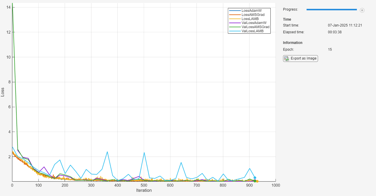
Initialize the TrainingProgressMonitor object. Because the timer starts when you create the monitor object, make sure that you create the object close to the training loop.

monitor = trainingProgressMonitor( ... Metrics=["LossAdamW", "LossAMSGrad", "LossLAMB",... "ValLossAdamW", "ValLossAMSGrad", "ValLossLAMB"], ... Info="Epoch", ... XLabel="Iteration"); groupSubPlot(monitor,"Loss",["LossAdamW", "LossAMSGrad", "LossLAMB","ValLossAdamW", "ValLossAMSGrad", "ValLossLAMB"])

Train the network using a custom training loop. For each epoch, shuffle the data and loop over mini-batches of data. For each mini-batch:

• Evaluate the model loss, gradients, and state using the dlfeval and modelLoss functions and update the network state.
• Update the network parameters using the custom solvers.
• Update the loss and epoch values in the training progress monitor.
• Stop if the Stop property is true. The Stop property value of the TrainingProgressMonitor object changes to true when you click the Stop button.

epoch = 0; iteration = 0;

netAdamW = net; netAMSGrad = net; netLAMB = net;

% Loop over epochs. while epoch < numEpochs && ~monitor.Stop

epoch = epoch + 1;

% Shuffle data.
shuffle(mbq);

% Loop over mini-batches.
while hasdata(mbq) && ~monitor.Stop

    iteration = iteration + 1;

    % Read mini-batch of data.
    [X,T] = next(mbq);

    % Evaluate the model gradients, state, and loss using dlfeval and the
    % modelLoss function and update the network state.
    [lossAdamW,gradientsAdamW,stateAdamW] = dlfeval(@modelLoss,netAdamW,X,T);
    [lossAMSGrad,gradientsAMSGrad,stateAMSGrad] = dlfeval(@modelLoss,netAMSGrad,X,T);
    [lossLAMB,gradientsLAMB,stateLAMB] = dlfeval(@modelLoss,netLAMB,X,T);

    netAdamW.State = stateAdamW;
    netAMSGrad.State = stateAMSGrad;
    netLAMB.State = stateLAMB;

    % Update the network parameters using different solvers.
    [netAdamW,avgGradAdamW,avgSqGradAdamW] = ...
        adamwupdate(netAdamW,avgGradAdamW,avgSqGradAdamW,gradientsAdamW,...
        iteration,learnRate,...
        gradDecay,sqGradDecay,...
        weightDecay,epsilon);

    [netAMSGrad,avgGradAMSGrad,avgSqGradAMSGrad,avgSqGradMaxAMSGrad] = ...
        amsgradupdate(netAMSGrad,avgGradAMSGrad,avgSqGradAMSGrad,...
        avgSqGradMaxAMSGrad,gradientsAMSGrad,...
        iteration,learnRate,...
        gradDecay,sqGradDecay,epsilon);

    [netLAMB,avgGradLAMB,avgSqGradLAMB] = ...
        lambupdate(netLAMB,avgGradLAMB,avgSqGradLAMB,gradientsLAMB,...
        iteration,learnRate,...
        gradDecay,sqGradDecay,...
        weightDecay,epsilon);

    % Evaluate the validation loss for training progress monitor every
    % validationFrequency iterations.
    if mod(iteration,validationFrequency) == 1
        valAdamW = testnet(netAdamW,augimdsValidation,["crossentropy","accuracy"]);
        valAMSGrad = testnet(netAMSGrad,augimdsValidation,["crossentropy","accuracy"]);
        valLAMB = testnet(netLAMB,augimdsValidation,["crossentropy","accuracy"]);
        recordMetrics(monitor,iteration,ValLossAdamW=valAdamW(1),ValLossAMSGrad=valAMSGrad(1),ValLossLAMB=valLAMB(1));

        % Track validation accuracy for comparison.
        accuracyValidationAdamW(ceil(iteration/validationFrequency)+1) = valAdamW(2);
        accuracyValidationAMSGrad(ceil(iteration/validationFrequency)+1) = valAMSGrad(2);
        accuracyValidationLAMB(ceil(iteration/validationFrequency)+1) = valLAMB(2);
    end

    % Update the training progress monitor.
    recordMetrics(monitor,iteration,LossAdamW=lossAdamW,LossAMSGrad=lossAMSGrad,LossLAMB=lossLAMB);
    updateInfo(monitor,Epoch=epoch);
    monitor.Progress = 100 * iteration/numIterations;
end

end

Test Model

Test the neural networks using the testnet function.

accuracyAdamW = testnet(netAdamW,augimdsTest,"accuracy")

accuracyAMSGrad = testnet(netAMSGrad,augimdsTest,"accuracy")

accuracyAMSGrad = 94.8000

accuracyLAMB = testnet(netLAMB,augimdsTest,"accuracy")

Compare Validation Accuracy

Compute the validation accuracy of all three networks after training.

accuracyValidationAdamW(end) = testnet(netAdamW,augimdsValidation,"accuracy"); accuracyValidationAMSGrad(end) = testnet(netAMSGrad,augimdsValidation,"accuracy"); accuracyValidationLAMB(end) = testnet(netLAMB,augimdsValidation,"accuracy");

For each of the solvers, plot the epoch numbers against the validation accuracy.

accuracyValidation = [ accuracyValidationAdamW,... accuracyValidationAMSGrad,... accuracyValidationLAMB];

figure iteration = [0 1:validationFrequency:numIterations numIterations]; plot(iteration,accuracyValidation) ylim([0 100]) title("Validation Accuracy") xlabel("Iteration") ylabel("Validation Accuracy") legend(["AdamW" "AMSGrad" "LAMB"],Location="southeast")

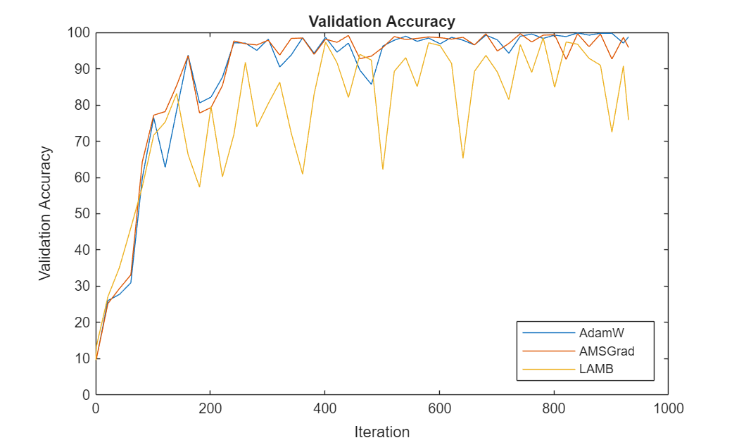
This plot shows how the progression of validation accuracy for each solver across the epochs.

Bibliography

1. Loshchilov, Ilya, and Frank Hutter. "Decoupled Weight Decay Regularization." arXiv preprint arXiv:1711.05101 (2017).
2. Reddi, Sashank J., et al. "On the Convergence of Adam and Beyond." International Conference on Learning Representations (ICLR), 2018.
3. You, Yang, et al. "Large Batch Optimization for Deep Learning: Training BERT in 76 Minutes." arXiv preprint arXiv:1904.00962 (2019).

See Also

trainingProgressMonitor | dlarray | dlgradient | dlfeval | dlnetwork | forward | predict | minibatchqueue | onehotdecode

Topics

• Define Model Loss Function for Custom Training Loop
• Define Custom Training Loops, Loss Functions, and Networks
• Specify Training Options in Custom Training Loop
• Monitor Custom Training Loop Progress
• List of Deep Learning Layers
• List of Functions with dlarray Support