Detect Vanishing Gradients in Deep Neural Networks by Plotting Gradient Distributions - MATLAB & Simulink (original) (raw)
This example shows how to monitor vanishing gradients while training a deep neural network.
A common problem in deep network training is vanishing gradients. Deep learning training algorithms aim to minimize the loss by adjusting the learnable parameters of the network during training. Gradient-based training algorithms determine the level of adjustment using the gradients of the loss function with respect to the current learnable parameters. For earlier layers, the gradient computation uses the propagated gradients from the previous layers. Therefore, when a network contains activation functions that always produce gradient values less than 1, the value of the gradients can become increasingly small as the updating algorithm moves towards the initial layers. As a result, early layers in the network can receive a gradient that is vanishingly small and, therefore, the network is unable to learn. However, if the gradient of the activation function is always greater than or equal to 1, the gradients can flow through the network, reducing the chance of vanishing gradients.
This example trains two networks with different activation functions and compares their gradient distributions.
Compare Activation Functions
To illustrate the different properties of activation functions, compare two common deep learning activation functions: ReLU and sigmoid.
ReLU(x)={xx≥00x<0
Sigmoid(x)=(1+exp(-x))-1
Evaluate the gradients of the ReLU and sigmoid activation functions.
x = linspace(-5,5,1000);
reluActivation = max(0,x); reluGradient = gradient(reluActivation,0.01);
sigmoidActivation = 1./(1 + exp(-x)); sigmoidGradient = gradient(sigmoidActivation,0.01);
Plot the ReLU and sigmoid activation functions and their gradients.
figure tiledlayout(1,2)
nexttile plot(x,[reluActivation;reluGradient]) legend("ReLU","Gradient of ReLU")
nexttile plot(x,[sigmoidActivation;sigmoidGradient]) legend("Sigmoid","Gradient of Sigmoid")

The ReLU gradient is either 0 or 1 for the entire range. Therefore, the gradient does not become increasingly small as it backpropagates through the network, reducing the chance of vanishing gradients. The sigmoid gradient curve is less than 1 for the entire range. Therefore, a network containing sigmoid activation layers can suffer from the vanishing gradient problem.
Load Data
Load sample data consisting of 5000 synthetic images of handwritten digits and their labels using digitTrain4DArrayData.
[XTrain,TTrain] = digitTrain4DArrayData; numObservations = length(TTrain);
To automatically resize the training images, use an augmented image datastore.
inputSize = [28,28,1]; augimdsTrain = augmentedImageDatastore(inputSize(1:2),XTrain,TTrain);
Determine the number of classes in the training data.
classes = categories(TTrain); numClasses = numel(classes);
Define Network
To compare the effect of the activation layer, construct two networks. Each network contains either ReLU or sigmoid activation layers separating four fully connected layers. By comparing the training progress of these two networks, you can see the impact of the activation layer during training. These networks are for demonstration purposes only. For an example showing how to create and train a simple image classification network, see Create Simple Deep Learning Neural Network for Classification.
activationTypes = ["ReLU","Sigmoid"]; numNetworks = length(activationTypes);
for i = 1:numNetworks activationType = activationTypes(i);
switch activationType
    case "ReLU"
        activationLayer = reluLayer;
    case "Sigmoid"
        activationLayer = sigmoidLayer;
end

layers = [
    imageInputLayer(inputSize,Normalization="none")
    fullyConnectedLayer(10)
    activationLayer
    fullyConnectedLayer(10)
    activationLayer
    fullyConnectedLayer(10)
    activationLayer
    fullyConnectedLayer(numClasses)
    softmaxLayer];

% Create a dlnetwork object from the layers.
networks{i} = dlnetwork(layers);
end
Define Model Loss Function
Create the function modelLoss, listed at the end of the example, which takes as input a dlnetwork object and a mini-batch of input data with corresponding labels and returns the loss and the gradients of the loss with respect to the learnable parameters in the network.
Specify Training Options
Train for 50 epochs with a mini-batch size of 128.
numEpochs = 50; miniBatchSize = 128;
Train Models
To compare the two networks, track the loss and average gradients for each layer in each network. Each network contains four learnable layers.
numIterations = numEpochs*ceil(numObservations/miniBatchSize); numLearnableLayers = 4;
losses = zeros(numIterations,numNetworks); meanGradients = zeros(numIterations,numNetworks,numLearnableLayers);
Create a minibatchqueue object that processes and manages mini-batches of images during training. For each mini-batch:
- Use the custom mini-batch preprocessing function
preprocessMiniBatch, defined at the end of this example, to convert the labels to one-hot encoded variables. - Format the image data with the dimension labels
"SSCB"(spatial, spatial, channel, batch). By default, theminibatchqueueobject converts the data todlarrayobjects with underlying type single. Do not add a format to the class labels. - Train on a GPU if one is available. By default, the
minibatchqueueobject converts each output to agpuArrayif a GPU is available. Using a GPU requires Parallel Computing Toolbox™ and a supported GPU device. For information on supported devices, see GPU Computing Requirements (Parallel Computing Toolbox).
mbq = minibatchqueue(augimdsTrain,... MiniBatchSize=miniBatchSize,... MiniBatchFcn=@preprocessMiniBatch,... MiniBatchFormat=["SSCB",""]);
Loop over each of the networks. For each network:
- Find the indices of the weights and the names of the layers with weights.
- Initialize the plots of the weight distributions using the supporting function setupGradientDistributionAxes, defined at the end of this example.
- Train the network using a custom training loop.
For each epoch of the custom training loop, shuffle the data and loop over mini-batches of data. For each mini-batch:
- Evaluate the model loss and gradients using the
dlfevalandmodelLossfunctions. - Update the network parameters using the
adamupdatefunction. - Save the average gradient value for each layer at each iteration.
At the end of each epoch, plot the gradient distributions of the weights for each learnable layer using the supporting function plotGradientDistributions, defined at the end of this example.
for activationIdx = 1:numNetworks
activationName =  activationTypes(activationIdx);
net = networks{activationIdx};

% Find the indices of the weight learnables.
weightIdx = ismember(net.Learnables.Parameter,"Weights");

% Find the names of the layers with weights.
weightLayerNames = join([net.Learnables.Layer(weightIdx),...
    net.Learnables.Parameter(weightIdx)]);

% Prepare axes to display the weight distributions for each epoch
% using the supporting function setupGradientDistributionAxes.
plotSetup = setupGradientDistributionAxes(activationName,weightLayerNames,numEpochs);

% Initialize parameters for the Adam training algorithm.
averageGrad = [];
averageSqGrad = [];

% Train the network using a custom training loop.
iteration = 0;
start = tic;

% Reset minibatchqueue to the start of the data.
reset(mbq);

% Loop over epochs.
for epoch = 1:numEpochs
    % Shuffle data.
    shuffle(mbq);

    % Loop over mini-batches.
    while hasdata(mbq)
        iteration = iteration + 1;

        % Read mini-batch of data.
        [X,T] = next(mbq);

        % Evaluate the model loss and gradients using dlfeval and the
        % modelLoss function.
        [loss,gradients] = dlfeval(@modelLoss,net,X,T);

        % Update the network parameters using the Adam optimizer.
        [net,averageGrad,averageSqGrad] = adamupdate(net,gradients,averageGrad,averageSqGrad,iteration);

        % Record the loss at every iteration.
        losses(iteration,activationIdx) = loss;

        % Record the average gradient of each learnable layer at each iteration.
        gradientValues = gradients.Value(weightIdx);
        for ii = 1:numLearnableLayers
            meanGradients(iteration,activationIdx,ii) = mean(gradientValues{ii},"all");
        end
    end

    % At the end of each epoch, plot the gradient distributions of the weights
    % of each learnable layer using the supporting function
    % plotGradientDistributions.
    gradientValues = gradients.Value(weightIdx);
    plotGradientDistributions(plotSetup,gradientValues,epoch)
end
end
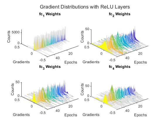

The gradient distribution plots show that the sigmoid network suffers from vanishingly small gradients. This effect becomes increasingly noticeable as the gradients flow back through the network toward the earlier layers.
Compare Losses
Compare the losses of the trained networks.
figure plot(losses) xlabel("Iteration") ylabel("Loss") legend(activationTypes)

The loss for the sigmoid network decreases slower than the loss for the ReLU network. Therefore, for this model, using ReLU activation layers results in faster learning.
Compare Mean Gradients
Compare the average gradient for each layer in each training iteration.
figure tiledlayout("flow") for ii = 1:numLearnableLayers nexttile plot(meanGradients(:,:,ii)) xlabel("Iteration") ylabel("Average Gradient") title(weightLayerNames(ii)) legend(activationTypes) end

The average gradient plot is consistent with the results seen in the gradient distribution plots. For the network with sigmoid layers, the range of values for the gradients is very small and centered around 0. In comparison, the network with ReLU layers has a much wider range of gradients, reducing the chance of vanishing gradients and increasing the rate of learning.
Supporting Functions
Model Loss Function
The modelLoss function takes as input the dlnetwork object net and a mini-batch of input data X with corresponding targets T containing the labels, and returns the loss and the gradients of the loss with respect to the learnable parameters.
function [loss,gradients] = modelLoss(net,X,T) Y = forward(net,X);
loss = crossentropy(Y,T); gradients = dlgradient(loss,net.Learnables); end
Mini Batch Preprocessing Function
The preprocessMiniBatch function preprocesses a mini-batch of predictors and labels using the following steps:
- Preprocess the images using the
preprocessMiniBatchPredictorsfunction. - Extract the label data from the incoming cell array and concatenate the data into a categorical array along the second dimension.
- One-hot encode the categorical labels into numeric arrays. Encoding into the first dimension produces an encoded array that matches the shape of the network output.
function [X,T] = preprocessMiniBatch(XCell,TCell) % Preprocess predictors. X = preprocessMiniBatchPredictors(XCell);
% Extract label data from cell and concatenate. T = cat(2,TCell{1:end});
% One-hot encode labels. T = onehotencode(T,1); end
Mini-Batch Predictors Preprocessing Function
The preprocessMiniBatchPredictors function preprocesses a mini-batch of predictors by extracting the image data from the input cell array and concatenating it into a numeric array. For grayscale input, concatenating over the fourth dimension adds a third dimension to each image to use as a singleton channel dimension.
function X = preprocessMiniBatchPredictors(XCell) % Concatenate. X = cat(4,XCell{1:end}); end
Calculate Distribution
The gradientDistributions function computes the histogram values and returns the bin centers and histogram counts.
function [centers,counts] = gradientDistributions(values) % Get the histogram count for the values. [counts,edges] = histcounts(values,30);
% histcounts returns edges of the bins. To get the bin centers, % calculate the midpoints between consecutive elements of the edges. centers = edges(1:end-1) + diff(edges)/2; end
Create Gradient Distribution Plot Axes
The setupGradientDistributionAxes function creates axes suitable for plotting the gradient distribution plots in 3-D. This function returns a structure array containing a TiledChartLayout object and a colormap that act as input to the plotGradientDistributions supporting function.
function plotSetup = setupGradientDistributionAxes(activationName,weightLayerNames,numEpochs) f = figure; t = tiledlayout(f,"flow",TileSpacing="tight"); t.Title.String = "Gradient Distributions with " + activationName + " Layers";
% To avoid updating the same values every epoch, set up axis % information before the training loop. for i = 1 : numel(weightLayerNames) tiledAx = nexttile(t,i);
% Set up the label names and titles.
xlabel(tiledAx,"Gradients");
ylabel(tiledAx,"Epochs");
zlabel(tiledAx,"Counts");
title(tiledAx,weightLayerNames(i));

% Rotate the view.
view(tiledAx, [-130, 50]);
xlim(tiledAx,[-0.5,0.5]);
ylim(tiledAx,[1,Inf]);
end
plotSetup.ColorMap = parula(numEpochs); plotSetup.TiledLayout = t; end
Plot Gradient Distributions
The plotGradientDistributions function takes as input a structure array containing a TiledChartLayout object and a colormap, and an array of values (for example, layer gradients) at a specific epoch, and plots smoothed histograms in 3-D. Use the supporting function setupGradientDistributionAxes to generate a suitable structure array input.
function plotGradientDistributions(plotSetup,gradientValues,epoch)
for w = 1:numel(gradientValues) nexttile(plotSetup.TiledLayout,w) color = plotSetup.ColorMap(epoch,:);
values = extractdata(gradientValues{w});

% Get the centers and counts for the distribution.
[centers,counts] = gradientDistributions(values);

% Plot the gradient values on the x axis, the epochs on the y axis, and the
% counts on the z axis. Set the edge color as white to more easily distinguish
% between the different histograms.
hold("on");
fill3(centers,zeros(size(counts))+epoch,counts,color,EdgeColor="#D9D9D9");
hold("off")
drawnow
end end
See Also
dlfeval | adamupdate | dlnetwork | minibatchqueue