filter - 1-D digital filter - MATLAB (original) (raw)

Syntax

Description

[y](#bt%5Fvs4t-1-y) = filter([b](#bt%5Fvs4t-1-b),[a](#bt%5Fvs4t-1-a),[x](#bt%5Fvs4t-1-x)) filters the input data x using a rational transfer function defined by the numerator and denominator coefficients b and a.

If a(1) is not equal to 1, then filter normalizes the filter coefficients by a(1). Therefore, a(1) must be nonzero.

If x is a vector, then filter returns the filtered data as a vector of the same size as x.
If x is a matrix, then filter acts along the first dimension and returns the filtered data for each column.
If x is a multidimensional array, then filter acts along the first array dimension whose size does not equal 1.

example

[y](#bt%5Fvs4t-1-y) = filter([b](#bt%5Fvs4t-1-b),[a](#bt%5Fvs4t-1-a),[x](#bt%5Fvs4t-1-x),[zi](#bt%5Fvs4t-1-zi)) uses initial conditions zi for the filter delays. The length of zi must equalmax(length(a),length(b))-1.

example

[y](#bt%5Fvs4t-1-y) = filter([b](#bt%5Fvs4t-1-b),[a](#bt%5Fvs4t-1-a),[x](#bt%5Fvs4t-1-x),[zi](#bt%5Fvs4t-1-zi),[dim](#bt%5Fvs4t-1-dim)) acts along dimension dim. For example, if x is a matrix, then filter(b,a,x,zi,2) returns the filtered data for each row.

example

[[y](#bt%5Fvs4t-1-y),[zf](#bt%5Fvs4t-1-zf)] = filter(___) also returns the final conditionszf of the filter delays, using any of the previous syntaxes.

example

Examples

collapse all

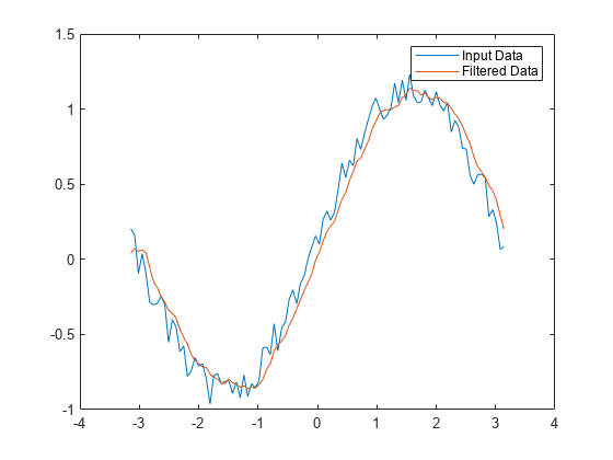
A moving-average filter is a common method used for smoothing noisy data. This example uses the filter function to compute averages along a vector of data.

Create a 1-by-100 row vector of sinusoidal data that is corrupted by random noise.

t = linspace(-pi,pi,100); rng default %initialize random number generator x = sin(t) + 0.25*rand(size(t));

A moving-average filter slides a window of length windowSize along the data, computing averages of the data contained in each window. The following difference equation defines a moving-average filter of a vector x:

y(n)=1windowSize(x(n)+x(n-1)+...+x(n-(windowSize-1))).

For a window size of 5, compute the numerator and denominator coefficients for the rational transfer function.

windowSize = 5; b = (1/windowSize)*ones(1,windowSize); a = 1;

Find the moving average of the data and plot it against the original data.

y = filter(b,a,x);

plot(t,x) hold on plot(t,y) legend('Input Data','Filtered Data')

Figure contains an axes object. The axes object contains 2 objects of type line. These objects represent Input Data, Filtered Data.

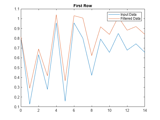
This example filters a matrix of data with the following rational transfer function.

H(z)=b(1)a(1)+a(2)z-1=11-0.2z-1

Create a 2-by-15 matrix of random input data.

rng default %initialize random number generator x = rand(2,15);

Define the numerator and denominator coefficients for the rational transfer function.

Apply the transfer function along the second dimension of x and return the 1-D digital filter of each row. Plot the first row of original data against the filtered data.

y = filter(b,a,x,[],2);

t = 0:length(x)-1; %index vector

plot(t,x(1,:)) hold on plot(t,y(1,:)) legend('Input Data','Filtered Data') title('First Row')

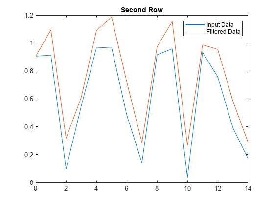
Figure contains an axes object. The axes object with title First Row contains 2 objects of type line. These objects represent Input Data, Filtered Data.

Plot the second row of input data against the filtered data.

figure plot(t,x(2,:)) hold on plot(t,y(2,:)) legend('Input Data','Filtered Data') title('Second Row')

Figure contains an axes object. The axes object with title Second Row contains 2 objects of type line. These objects represent Input Data, Filtered Data.

Define a moving-average filter with a window size of 3.

windowSize = 3; b = (1/windowSize)*ones(1,windowSize); a = 1;

Find the 3-point moving average of a 1-by-6 row vector of data.

x = [2 1 6 2 4 3]; y = filter(b,a,x)

y = 1×6

0.6667    1.0000    3.0000    3.0000    4.0000    3.0000

By default, the filter function initializes the filter delays as zero, assuming that both past inputs and outputs are zero. In this case, the first two elements of y are the 3-point moving average of the first element and the first two elements of x, respectively. In other words, the first element 0.6667 is the 3-point average of 2, and the second element 1 is the 3-point average of 2 and 1.

To include additional past inputs and outputs in your data, specify the initial conditions as the filter delays. These initial conditions for the present inputs are the final conditions that are obtained from applying the same transfer function to the past inputs (and past outputs). For example, include past inputs of [1 3]. Without filter delays, the past outputs are (0+0+1)/3 and (0+1+3)/3.

x_past = [1 3]; y_past = filter(b,a,x_past)

y_past = 1×2

0.3333    1.3333

However, you can continue applying the same transfer function to generate further nonzero outputs, assuming that the tails of these past inputs are zero. These further outputs are (1+3+0)/3 and (3+0+0)/3, which represent the final conditions obtained from the past inputs. To compute these final conditions, specify the second output argument of the filter function.

[y_past,zf] = filter(b,a,x_past)

y_past = 1×2

0.3333    1.3333

To include the past inputs in the present data, specify the filter delays by using the fourth input argument of the filter function. Use the final conditions from the past data as the initial conditions for the present data.

y = 1×6

2.0000    2.0000    3.0000    3.0000    4.0000    3.0000

In this case, the first element of y becomes the 3-point moving average of 1, 3, and 2, which is 2, and the second element of y becomes the moving average of 3, 2, and 1, which is 2.

Use initial and final conditions for filter delays to filter data in sections, especially if memory limitations are a consideration.

Generate a large random data sequence and split it into two segments, x1 and x2.

x = randn(10000,1);

x1 = x(1:5000); x2 = x(5001:end);

The whole sequence, x, is the vertical concatenation of x1 and x2.

Define the numerator and denominator coefficients for the rational transfer function,

H(z)=b(1)+b(2)z-1a(1)+a(2)z-1=2+3z-11+0.2z-1.

Filter the subsequences x1 and x2 one at a time. Output the final conditions from filtering x1 to store the internal status of the filter at the end of the first segment.

[y1,zf] = filter(b,a,x1);

Use the final conditions from filtering x1 as initial conditions to filter the second segment, x2.

y1 is the filtered data from x1, and y2 is the filtered data from x2. The entire filtered sequence is the vertical concatenation of y1 and y2.

Filter the entire sequence simultaneously for comparison.

y = filter(b,a,x);

isequal(y,[y1;y2])

Input Arguments

collapse all

Input data, specified as a vector, matrix, or multidimensional array.

Initial conditions for filter delays, specified as a vector, matrix, or multidimensional array.

If zi is a vector, then its length must be max(length(a),length(b))-1.
If zi is a matrix or multidimensional array, then the size of the leading dimension must bemax(length(a),length(b))-1. The size of each remaining dimension must match the size of the corresponding dimension of x. For example, consider using filter along the second dimension (dim = 2) of a 3-by-4-by-5 arrayx. The array zi must have size[max(length(a),length(b))-1]-by-3-by-5.

The default value, specified by [], initializes all filter delays to zero.

Dimension to operate along, specified as a positive integer scalar. If you do not specify the dimension, then the default is the first array dimension whose size does not equal 1.

Consider a two-dimensional input array, x.

If dim = 1, then filter(b,a,x,zi,1) operates along the columns of x and returns the filter applied to each column.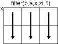
If dim = 2, then filter(b,a,x,zi,2) operates along the rows of x and returns the filter applied to each row.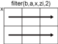

If dim is greater than ndims(x), thenfilter considers x as if it has additional dimensions up to dim with sizes of 1. For example, if x is a matrix with a size of 2-by-3 anddim = 3, then filter operates along the third dimension of x as if it has the size of 2-by-3-by-1.

Output Arguments

collapse all

Filtered data, returned as a vector, matrix, or multidimensional array of the same size as the input data, x.

If x is of type single, then filter natively computes in single precision, and y is also of type single. Otherwise, y is returned as type double.

Data Types: double | single

Final conditions for filter delays, returned as a vector, matrix, or multidimensional array.

If x is a vector, then zf is a column vector of length max(length(a),length(b))-1.
If x is a matrix or multidimensional array, then zf is an array of column vectors of lengthmax(length(a),length(b))-1, such that the number of columns in zf is equivalent to the number of columns in x. For example, consider using filter along the second dimension (dim = 2) of a 3-by-4-by-5 arrayx. The array zf has size[max(length(a),length(b))-1]-by-3-by-5.

Data Types: double | single

More About

collapse all

The input-output description of the filter operation on a vector in the Z-transform domain is a rational transfer function. A rational transfer function is of the form

which handles both finite impulse response (FIR) and infinite impulse response (IIR) filters [1]. Here,X(z) is the Z-transform of the input signal_x_, Y(z) is the Z-transform of the output signal y,na is the feedback filter order, and nb is the feedforward filter order. Due to normalization, assume a(1) = 1.

For a discrete signal with L elements, you can also express the rational transfer function as the difference equation

Furthermore, you can represent the rational transfer function using its direct-form II transposed implementation, as in the following diagram of an IIR digital filter. In the diagram, _na = nb = n–_1. If your feedback and feedforward filter orders are different, or na ≠ nb, then you can treat the higher-order terms as 0. For example, for a filter with a = [1,2] and b = [2,3,2,4], you can assume a = [1,2,0,0].

The operation of filter at a sample point m is given by the time-domain difference equations

By default, the filter function initializes the filter delays as zero, where w k(0) = 0. This initialization assumes both past inputs and outputs to be zero. To include nonzero past inputs in the present data, specify the initial conditions of the present data as the filter delays. You can consider the filter delays to be the final conditions that are obtained from applying the same transfer function to the past inputs (and past outputs). You can specify the fourth input argument zi when using filter to set the filter delays, where w k(0) =zi(k). You can also specify the second output argument zf when using filter to access the final conditions, where w k(L) = zf(k).

Tips

To use the filter function with the b coefficients from an FIR filter, use y = filter(b,1,x).
If you have Signal Processing Toolbox™, use y = filter(d,x) to filter an input signalx with a digitalFilter (Signal Processing Toolbox) objectd. To generate d based on frequency-response specifications, use designfilt (Signal Processing Toolbox).
See Digital Filtering (Signal Processing Toolbox) for more on filtering functions.

References

[1] Oppenheim, Alan V., Ronald W. Schafer, and John R. Buck. Discrete-Time Signal Processing. Upper Saddle River, NJ: Prentice-Hall, 1999.

Extended Capabilities

expand all

Thefilter function supports tall arrays with the following usage notes and limitations:

The two-output syntax [y,zf] = filter(___) is not supported whendim > 1.
When you use y = filter(d,x) with a digitalFilter (Signal Processing Toolbox) object d, the filter function does not support tall array for the input signal x.

For more information, see Tall Arrays.

Usage notes and limitations:

For input arguments b and a:
- You must specify the input vector as a fixed-size or variable-length vector at code generation time. Either the first or the second dimension of the vector can be variable size. All other dimensions must have a fixed size of 1.
For input argument x:
- If you do not specify a dimension, the code generator operates along the first dimension of the input array that is variable size or whose size does not equal 1. If this dimension is variable size at code generation time and is 1 at run time, a run-time error can occur. To avoid this error, specify the dimension.
If used, the dim argument must be a constant at code generation time.

Usage notes and limitations:

The arguments b and a must be vectors at code generation time. This means that at least one of the first two dimensions of each argument must have a fixed size of 1.
Input argument
If you do not specify a dimension, the code generator operates along the first dimension of the input array that is variable size or whose size does not equal 1. If this dimension is variable size at code generation time and is 1 at run time, a run-time error can occur. To avoid this error, specify the dimension.
If used, the dim argument must be a constant at code generation time.

The filter function fully supports GPU arrays. To run the function on a GPU, specify the input data as a gpuArray (Parallel Computing Toolbox). For more information, see Run MATLAB Functions on a GPU (Parallel Computing Toolbox).

You can also apply a 1-D digital filter on the GPU using the y = filter(d,x) syntax, where d is a digitalFilter (Signal Processing Toolbox) object andx is a gpuArray. It is not necessary to convert the coefficients of the digitalFilter object to agpuArray.

Version History

Introduced before R2006a