line - Create primitive line - MATLAB (original) (raw)

Syntax

Description

line([x](#buzqtg4-x),[y](#buzqtg4-y)) plots a line in the current axes using the data in vectors x andy. If either x ory, or both are matrices, then line draws multiple lines. Unlike the plot function,line adds the line to the current axes without deleting other graphics objects or resetting axes properties.

example

line([x](#buzqtg4-x),[y](#buzqtg4-y),[z](#buzqtg4-z)) plots a line in three-dimensional coordinates.

example

line draws a line from the point (0,0) to (1,1) with the default property settings.

line(___,[Name,Value](#namevaluepairarguments)) modifies the appearance of the line using one or more name-value argument pairs. For example,'LineWidth',3 sets the line width to 3 points. Specify name-value pairs after all other input arguments. If you specify the data using name-value pairs, for exampleline('XData',x,'YData',y), then you must specify vector data.

example

line([ax](#buzqtg4-ax),___) creates the line in the Cartesian, polar, or geographic axes specified by ax instead of in the current axes (gca). Specify ax as the first input argument.

[pl](#buzqtg4-pl) = line(___) returns all primitive Line objects created. Use pl to modify properties of a specific Line object after it is created. For a list, see Line Properties.

example

Examples

collapse all

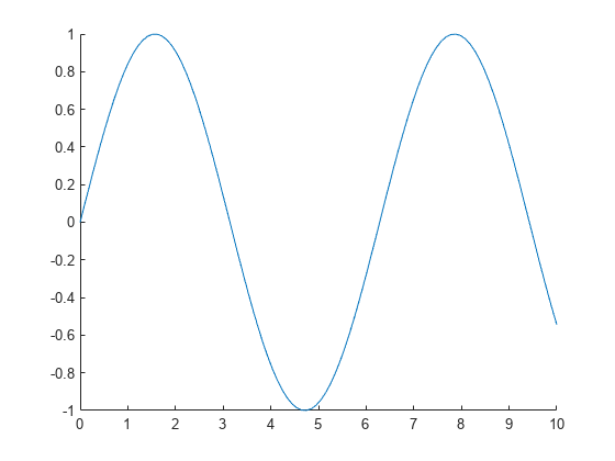
Create x and y as vectors. Then plot y versus x.

x = linspace(0,10); y = sin(x); line(x,y)

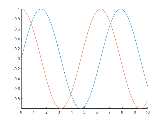
Plot two lines by specifying x and y as matrices. Use line to plot columns of y versus columns of x as separate lines.

x = linspace(0,10)'; y = [sin(x) cos(x)]; line(x,y)

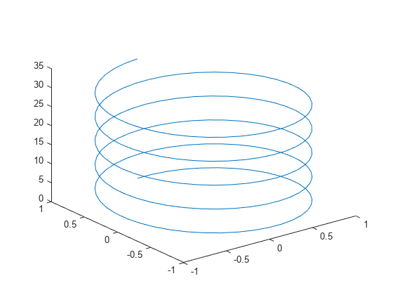
Plot a line in 3-D coordinates by specifying x, y, and z values. Change the axes to a 3-D view using view(3).

t = linspace(0,10*pi,200); x = sin(t); y = cos(t); z = t; line(x,y,z) view(3)

Create x and y as vectors. Then call the low-level version of the line function by specifying the data as name-value pair arguments. When you call the function this way, the resulting line is black.

x = linspace(0,10); y = sin(x); line('XData',x,'YData',y)

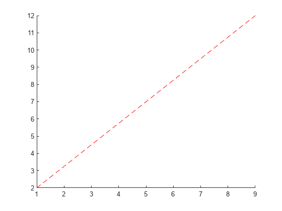
Draw a red, dashed line between the points (1,2) and (9,12). Set the Color and LineStyle properties as name-value pairs.

x = [1 9]; y = [2 12]; line(x,y,'Color','red','LineStyle','--')

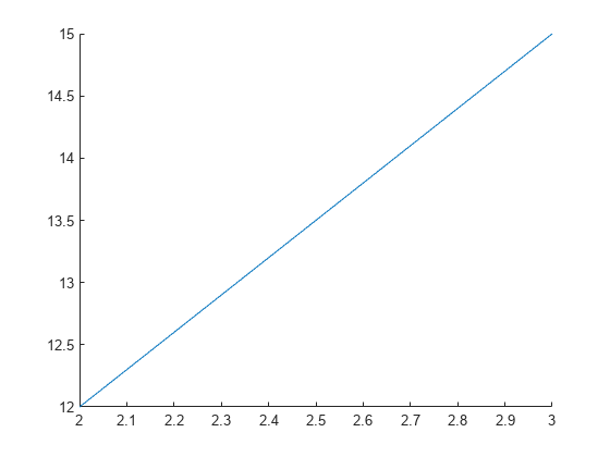
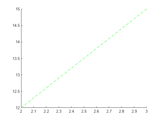
First, draw a line from the point (3,15) to (2,12) and return the Line object. Then change the line to a green, dashed line. Use dot notation to set properties.

x = [3 2]; y = [15 12]; pl = line(x,y);

pl.Color = 'green'; pl.LineStyle = '--';

Input Arguments

collapse all

First coordinate, specified as a vector or a matrix. Matrix inputs are supported for Cartesian axes only.

The interpretation of the first coordinate depends on the type of axes. For Cartesian axes, the first coordinate is _x_-axis position in data units.

• If x and y are both vectors with the same length, then line plots a single line.
• If x and y are matrices with the same size, then line plots multiple lines. The function plots columns of y versusx.
• If one of x or y is a vector and the other is a matrix, then line plots multiple lines. The length of the vector must equal one of the matrix dimensions:
  • If the vector length equals the number of matrix rows, then line plots each matrix column versus the vector.
  • If the vector length equals the number of matrix columns, then line plots each matrix row versus the vector.
  • If the matrix is square, then line plots each column versus the vector.

For polar axes, the first coordinate is the polar angle_θ_ in radians. For geographic axes, the first coordinate is latitude in degrees. To plot lines in these types of axes,x and y must be the same size.

Example: x = linspace(0,10,25)

Data Types: single | double | int8 | int16 | int32 | int64 | uint8 | uint16 | uint32 | uint64 | categorical | datetime | duration

Second coordinate, specified as a vector or a matrix. Matrix inputs are supported for Cartesian axes only.

The interpretation of the second coordinate depends on the type of axes. For Cartesian axes, the second coordinate is _y_-axis position in data units.

• If x and y are both vectors with the same length, then line plots a single line.
• If x and y are matrices with the same size, then line plots multiple lines. The function plots columns of y versusx.
• If one of x or y is a vector and the other is a matrix, then line plots multiple lines. The length of the vector must equal one of the matrix dimensions:
  • If the vector length equals the number of matrix rows, then line plots each matrix column versus the vector.
  • If the vector length equals the number of matrix columns, then line plots each matrix row versus the vector.
  • If the matrix is square, then line plots each column versus the vector.

For polar axes, the second coordinate is the radius in data units. For geographic axes, the second coordinate is longitude in degrees. To plot lines in these types of axes, x and y must be the same size.

Example: y = sin(x)

Data Types: single | double | int8 | int16 | int32 | int64 | uint8 | uint16 | uint32 | uint64 | categorical | datetime | duration

Third coordinate, specified as a vector or a matrix. Matrix inputs are supported for Cartesian axes only.

The interpretation of the third coordinate depends on the type of axes. For Cartesian axes, the third coordinate is _z_-axis position in data units.

• If x, y, andz are all vectors with the same length, then line plots a single 3-D line.
• If x, y, andz are all matrices with the same size, then line plots multiple 3-D lines using the matrix columns.
• If one or two of x, y, and z is a vector and the others are matrices of the same size, then line plots multiple 3-D lines. The length of the vector must equal one of the matrix dimensions.

For polar and geographic axes, the third coordinate affects the layering of 2-D lines on the axes. To use the third coordinate in these types of axes, x, y, and z must be the same size.

Example: z = sin(x) + cos(y)

Data Types: single | double | int8 | int16 | int32 | int64 | uint8 | uint16 | uint32 | uint64 | categorical | datetime | duration

Target axes, specified as an Axes object, aPolarAxes object, or aGeographicAxes object. If you do not specify the axes, then the line function plots in the current axes.

Name-Value Arguments

collapse all

Specify optional pairs of arguments asName1=Value1,...,NameN=ValueN, where Name is the argument name and Value is the corresponding value. Name-value arguments must appear after other arguments, but the order of the pairs does not matter.

Before R2021a, use commas to separate each name and value, and enclose Name in quotes.

Example: line(x,y,'Color','red','LineWidth',3) creates a red line that is 3 points wide.

The properties listed here are only a subset. For a full list, see Line Properties.

Line color, specified as an RGB triplet, a hexadecimal color code, a color name, or a short name.

For a custom color, specify an RGB triplet or a hexadecimal color code.

• An RGB triplet is a three-element row vector whose elements specify the intensities of the red, green, and blue components of the color. The intensities must be in the range [0,1], for example, [0.4 0.6 0.7].
• A hexadecimal color code is a string scalar or character vector that starts with a hash symbol (#) followed by three or six hexadecimal digits, which can range from 0 to F. The values are not case sensitive. Therefore, the color codes"#FF8800","#ff8800","#F80", and"#f80" are equivalent.

Alternatively, you can specify some common colors by name. This table lists the named color options, the equivalent RGB triplets, and the hexadecimal color codes.

Color Name	Short Name	RGB Triplet	Hexadecimal Color Code	Appearance
"red"	"r"	[1 0 0]	"#FF0000"
"green"	"g"	[0 1 0]	"#00FF00"
"blue"	"b"	[0 0 1]	"#0000FF"
"cyan"	"c"	[0 1 1]	"#00FFFF"
"magenta"	"m"	[1 0 1]	"#FF00FF"
"yellow"	"y"	[1 1 0]	"#FFFF00"
"black"	"k"	[0 0 0]	"#000000"
"white"	"w"	[1 1 1]	"#FFFFFF"
"none"	Not applicable	Not applicable	Not applicable	No color

This table lists the default color palettes for plots in the light and dark themes.

Palette	Palette Colors
"gem" — Light theme default_Before R2025a: Most plots use these colors by default._
"glow" — Dark theme default

You can get the RGB triplets and hexadecimal color codes for these palettes using the orderedcolors and rgb2hex functions. For example, get the RGB triplets for the "gem" palette and convert them to hexadecimal color codes.

RGB = orderedcolors("gem"); H = rgb2hex(RGB);

Before R2023b: Get the RGB triplets using RGB = get(groot,"FactoryAxesColorOrder").

Before R2024a: Get the hexadecimal color codes using H = compose("#%02X%02X%02X",round(RGB*255)).

Example: line(x,y,'Color','blue')

Example: line(x,y,'Color',[0.5 0.5 1])

Example: line(x,y,'Color','#D9A2E9')

Marker size, specified as a positive value in points, where 1 point = 1/72 of an inch.

Output Arguments

collapse all

Primitive line object. Use pl to query or modify properties of the line after it is created. For a list, see Line Properties.

Tips

• Unlike the plot function, the line function does not call newplot before plotting and does not respect the value of the NextPlot property for the figure or axes. It simply adds the line to the current axes without deleting other graphics objects or resetting axes properties. However, some axes properties, such as the axis limits, can update to accommodate the line.

Extended Capabilities

expand all

The line function supports GPU array input with these usage notes and limitations:

• This function accepts GPU arrays, but does not run on a GPU.

For more information, see Run MATLAB Functions on a GPU (Parallel Computing Toolbox).

Version History

Introduced before R2006a

expand all

Now that the SeriesIndex property is available for lines created with the line function, the lines cycle through the same colors (and optional line styles) that most other plots do.

The default color change applies only to the lines you create when you specify thex, y, and optional z arguments. If you create lines with a syntax that uses name-value arguments only, the plots look the same as in previous releases.

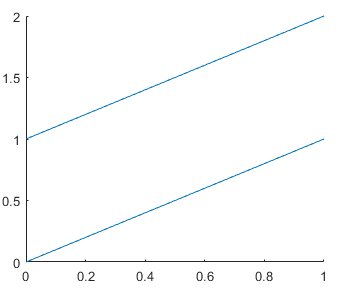
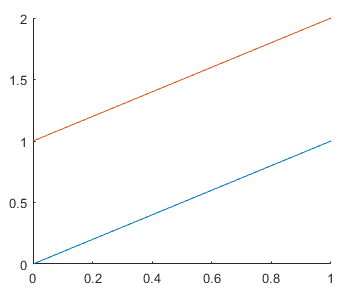
For example, create two lines with x and y input arguments. In R2023b, the first line is blue and the second line is red-orange. Before R2023b, both lines were blue.

line1 = line([0 1],[0 1]); line2 = line([0 1],[1 2]);

To preserve the behavior of previous releases, set theSeriesIndex property of the lines to 1. You can set the property using a name-value argument when you call theline function, or you can set the property of theLine object using dot notation later.

% Use a name-value argument line1 = line([0 1],[0 1],SeriesIndex=1);

% Use dot notation line2 = line([0 1],[1 2]); line2.SeriesIndex = 1;