Histogram - Histogram plot - MATLAB (original) (raw)

Description
Histograms are a type of bar plot that group data into bins. After you create a Histogram object, you can modify aspects of the histogram by changing its property values. This is particularly useful for quickly modifying the properties of the bins or changing the display.
Creation
Syntax
Description
histogram([X](#buhzm%5Fz-1-X)) creates a histogram plot of X. The histogram function uses an automatic binning algorithm that returns bins with a uniform width, chosen to cover the range of elements in X and reveal the underlying shape of the distribution. histogram displays the bins as rectangular bars such that the height of each rectangle indicates the number of elements in the bin.
histogram([X](#buhzm%5Fz-1-X),[nbins](#buhzm%5Fz-1-nbins)) specifies the number of bins.
histogram([X](#buhzm%5Fz-1-X),[edges](#buhzm%5Fz-1-edges)) sorts X into bins with bin edges specified in a vector.
histogram('BinEdges',[edges](#buhzm%5Fz-1-edges),'BinCounts',[counts](#buhzm%5Fz-1-counts)) plots the specified bin counts and does not do any data binning.
histogram([C](#buhzm%5Fz-1-C)) plots a histogram with a bar for each category in categorical arrayC.
histogram([C](#buhzm%5Fz-1-C),[Categories](#buhzm%5Fz-1%5Fsep%5Fshared-Categories)) plots only a subset of categories in C.
histogram('Categories',[Categories](#buhzm%5Fz-1%5Fsep%5Fshared-Categories),'BinCounts',[counts](#buhzm%5Fz-1-counts)) manually specifies categories and associated bin counts.histogram plots the specified bin counts and does not do any data binning.
histogram(___,[Name,Value](#namevaluepairarguments)) specifies additional parameters using one or more name-value arguments for any of the previous syntaxes. For example, specifyNormalization to use a different type of normalization. For a list of properties, see Histogram Properties.
histogram([ax](#buhzm%5Fz-1-ax),___) plots into the specified axes instead of into the current axes (gca). ax can precede any of the input argument combinations in the previous syntaxes.
[h](#buhzm%5Fz-1-h) = histogram(___) returns a Histogram object. Use this to inspect and adjust the properties of the histogram. For a list of properties, seeHistogram Properties.
Input Arguments
Data to distribute among bins, specified as a vector, matrix, or multidimensional array. histogram treats matrix and multidimensional array data as a single column vector,X(:), and plots a single histogram.
histogram ignores all NaN andNaT values. Similarly,histogram ignores Inf and-Inf values, unless the bin edges explicitly specify Inf or -Inf as a bin edge. Although NaN, NaT,Inf, and -Inf values are typically not plotted, they are still included in normalization calculations that include the total number of data elements, such as'probability'.
Note
If X contains integers of typeint64 or uint64 that are larger than flintmax, then it is recommended that you explicitly specify the histogram bin edges.histogram automatically bins the input data using double precision, which lacks integer precision for numbers greater than flintmax.
Data Types: single | double | int8 | int16 | int32 | int64 | uint8 | uint16 | uint32 | uint64 | logical | datetime | duration
Categorical data, specified as a categorical array.histogram does not plot undefined categorical values. However, undefined categorical values are still included in normalization calculations that include the total number of data elements, such as 'probability'.
Data Types: categorical
Number of bins, specified as a positive integer. If you do not specifynbins, then histogram determines the number of bins from the values inX.
If you specify nbins withBinMethod, BinWidth orBinEdges, histogram only honors the last parameter.
Example: histogram(X,15) creates a histogram with 15 bins.
Bin edges, specified as a vector. edges(1) is the leading edge of the first bin, and edges(end) is the trailing edge of the last bin.
Each bin includes the leading edge, but does not include the trailing edge, except for the last bin which includes both edges.
For datetime and duration data,edges must be a datetime orduration vector in monotonically increasing order.
If you specify counts, thenedges must be a row vector.
Data Types: single | double | int8 | int16 | int32 | int64 | uint8 | uint16 | uint32 | uint64 | logical | datetime | duration
Data Types: cell | categorical | string | pattern
Bin counts, specified as a vector. Use this input to pass bin counts to histogram when the bin counts calculation is performed separately and you do not want histogram to do any data binning.
The size of counts must be equal to the number of bins.
- For numeric histograms, the number of bins is
length(edges)-1. - For categorical histograms, the number of bins is equal to the number of categories.
Example: histogram('BinEdges',-2:2,'BinCounts',[5 8 15 9])
Example: histogram('Categories',{'Yes','No','Maybe'},'BinCounts',[22 18 3])
Target axes, specified as an Axes object or aPolarAxes object. If you do not specify the axes and if the current axes are Cartesian axes, then thehistogram function uses the current axes (gca). To plot into polar axes, specify thePolarAxes object as the first input argument or use the polarhistogram function.
Name-Value Arguments
Specify optional pairs of arguments asName1=Value1,...,NameN=ValueN, where Name is the argument name and Value is the corresponding value. Name-value arguments must appear after other arguments, but the order of the pairs does not matter.
Example: histogram(X,BinWidth=5)
Before R2021a, use commas to separate each name and value, and enclose Name in quotes.
Example: histogram(X,'BinWidth',5)
Bins
Categories
Data
Color and Styling
Transparency of histogram bar edges, specified as a scalar value in the range [0,1]. A value of1 means fully opaque and 0 means completely transparent (invisible).
Example: `histogram`(X,'EdgeAlpha',0.5) creates a histogram plot with semi-transparent bar edges.
Data Types: single | double | int8 | int16 | int32 | int64 | uint8 | uint16 | uint32 | uint64
Output Arguments
Properties
Object Functions
Examples
Generate 10,000 random numbers and create a histogram. The histogram function automatically chooses an appropriate number of bins to cover the range of values in x and show the shape of the underlying distribution.
x = randn(10000,1); h = histogram(x)
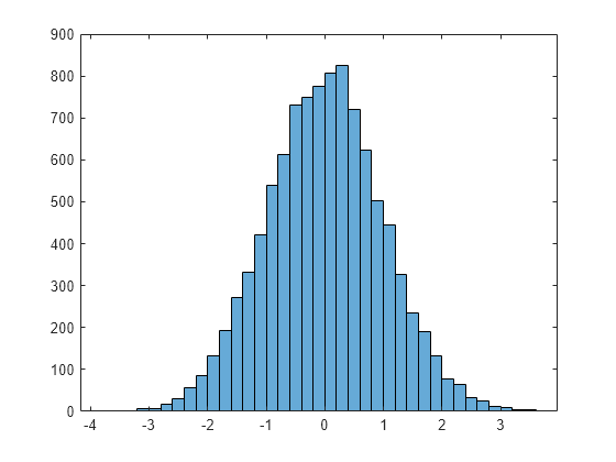
h = Histogram with properties:
         Data: [10000×1 double]
       Values: [2 2 1 6 7 17 29 57 86 133 193 271 331 421 540 613 730 748 776 806 824 721 623 503 446 326 234 191 132 78 65 33 26 11 8 5 5]
      NumBins: 37
     BinEdges: [-3.8000 -3.6000 -3.4000 -3.2000 -3 -2.8000 -2.6000 -2.4000 -2.2000 -2 -1.8000 -1.6000 -1.4000 -1.2000 -1 -0.8000 -0.6000 -0.4000 -0.2000 0 0.2000 0.4000 0.6000 0.8000 1.0000 1.2000 1.4000 1.6000 1.8000 2.0000 2.2000 … ] (1×38 double)
     BinWidth: 0.2000
    BinLimits: [-3.8000 3.6000]
Normalization: 'count'
    FaceColor: 'auto'
    EdgeColor: [0.1294 0.1294 0.1294]
Show all properties
When you specify an output argument to the histogram function, it returns a histogram object. You can use this object to inspect the properties of the histogram, such as the number of bins or the width of the bins.
Find the number of histogram bins.
Plot a histogram of 1,000 random numbers sorted into 25 equally spaced bins.
x = randn(1000,1); nbins = 25; h = histogram(x,nbins)
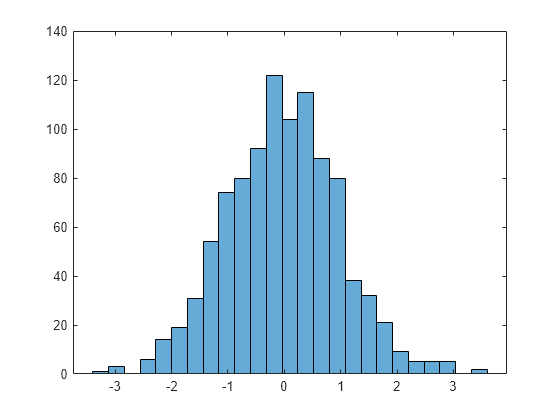
h = Histogram with properties:
         Data: [1000×1 double]
       Values: [1 3 0 6 14 19 31 54 74 80 92 122 104 115 88 80 38 32 21 9 5 5 5 0 2]
      NumBins: 25
     BinEdges: [-3.4000 -3.1200 -2.8400 -2.5600 -2.2800 -2 -1.7200 -1.4400 -1.1600 -0.8800 -0.6000 -0.3200 -0.0400 0.2400 0.5200 0.8000 1.0800 1.3600 1.6400 1.9200 2.2000 2.4800 2.7600 3.0400 3.3200 3.6000]
     BinWidth: 0.2800
    BinLimits: [-3.4000 3.6000]
Normalization: 'count'
    FaceColor: 'auto'
    EdgeColor: [0.1294 0.1294 0.1294]
Show all properties
Find the bin counts.
counts = 1×25
1 3 0 6 14 19 31 54 74 80 92 122 104 115 88 80 38 32 21 9 5 5 5 0 2Generate 1,000 random numbers and create a histogram.
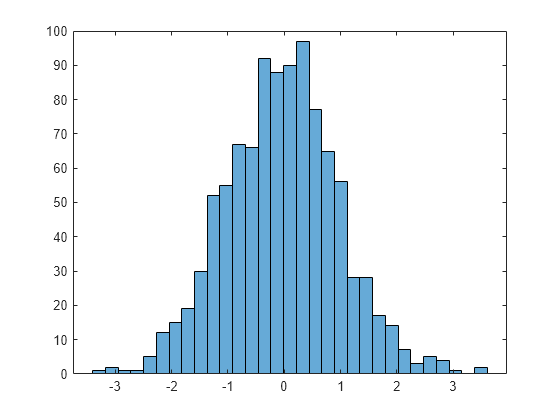
X = randn(1000,1); h = histogram(X)
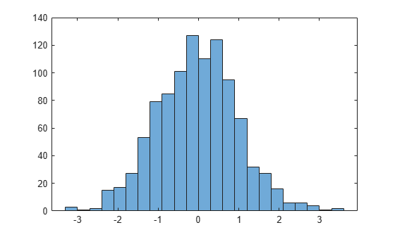
h = Histogram with properties:
         Data: [1000×1 double]
       Values: [3 1 2 15 17 27 53 79 85 101 127 110 124 95 67 32 27 16 6 6 4 1 2]
      NumBins: 23
     BinEdges: [-3.3000 -3.0000 -2.7000 -2.4000 -2.1000 -1.8000 -1.5000 -1.2000 -0.9000 -0.6000 -0.3000 0 0.3000 0.6000 0.9000 1.2000 1.5000 1.8000 2.1000 2.4000 2.7000 3 3.3000 3.6000]
     BinWidth: 0.3000
    BinLimits: [-3.3000 3.6000]
Normalization: 'count'
    FaceColor: 'auto'
    EdgeColor: [0.1294 0.1294 0.1294]
Show all properties
Use the morebins function to coarsely adjust the number of bins.
Nbins = morebins(h); Nbins = morebins(h)
Adjust the bins at a fine grain level by explicitly setting the number of bins.
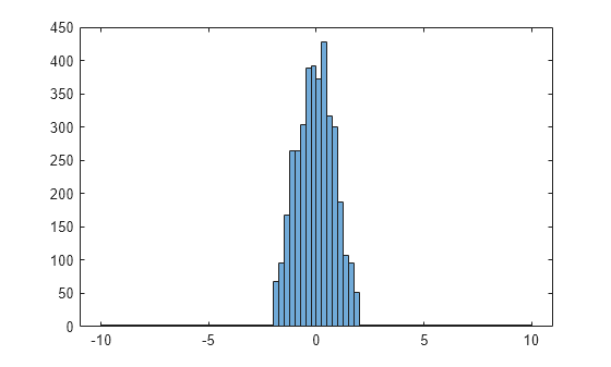
Generate 1,000 random numbers and create a histogram. Specify the bin edges as a vector with wide bins on the edges of the histogram to capture the outliers that do not satisfy |x|<2. The first vector element is the left edge of the first bin, and the last vector element is the right edge of the last bin.
x = randn(1000,1); edges = [-10 -2:0.25:2 10]; h = histogram(x,edges);
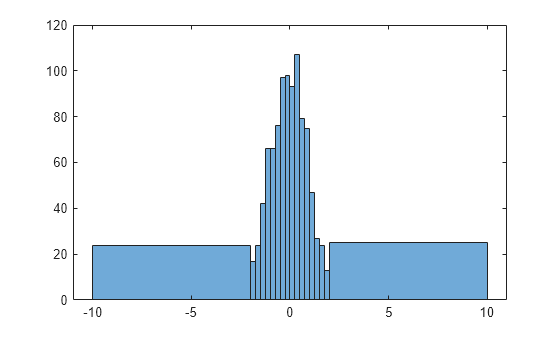
Specify the Normalization property as 'countdensity' to flatten out the bins containing the outliers. Now, the area of each bin (rather than the height) represents the frequency of observations in that interval.
h.Normalization = 'countdensity';
Create a categorical vector that represents votes. The categories in the vector are 'yes', 'no', or 'undecided'.
A = [0 0 1 1 1 0 0 0 0 NaN NaN 1 0 0 0 1 0 1 0 1 0 0 0 1 1 1 1]; C = categorical(A,[1 0 NaN],{'yes','no','undecided'})
C = 1×27 categorical no no yes yes yes no no no no undecided undecided yes no no no yes no yes no yes no no no yes yes yes yes
Plot a categorical histogram of the votes, using a relative bar width of 0.5.
h = histogram(C,'BarWidth',0.5)

h = Histogram with properties:
          Data: [no    no    yes    yes    yes    no    no    no    no    undecided    undecided    yes    no    no    no    yes    no    yes    no    yes    no    no    no    yes    yes    yes    yes]
        Values: [11 14 2]
NumDisplayBins: 3
    Categories: {'yes'  'no'  'undecided'}
  DisplayOrder: 'data'
 Normalization: 'count'
  DisplayStyle: 'bar'
     FaceColor: 'auto'
     EdgeColor: [0.1294 0.1294 0.1294]
Show all properties
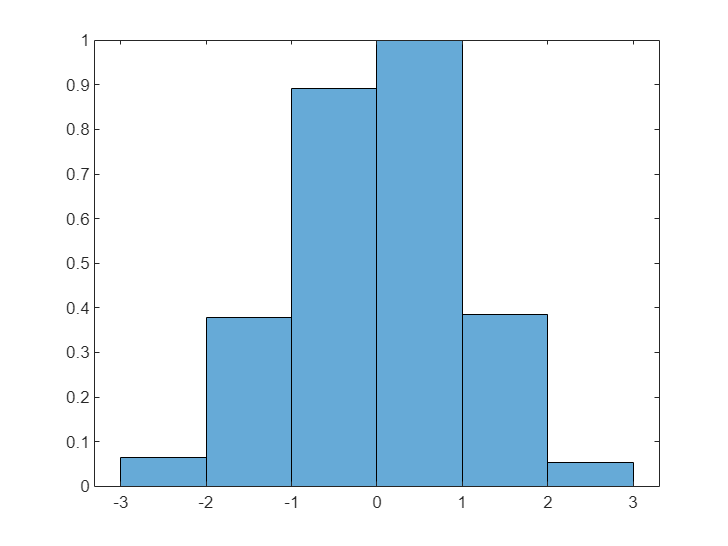
Generate 1,000 random numbers and create a histogram using the 'probability' normalization.
x = randn(1000,1); h = histogram(x,'Normalization','probability')
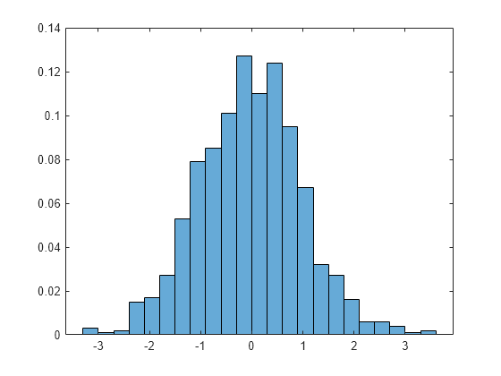
h = Histogram with properties:
         Data: [1000×1 double]
       Values: [0.0030 1.0000e-03 0.0020 0.0150 0.0170 0.0270 0.0530 0.0790 0.0850 0.1010 0.1270 0.1100 0.1240 0.0950 0.0670 0.0320 0.0270 0.0160 0.0060 0.0060 0.0040 1.0000e-03 0.0020]
      NumBins: 23
     BinEdges: [-3.3000 -3.0000 -2.7000 -2.4000 -2.1000 -1.8000 -1.5000 -1.2000 -0.9000 -0.6000 -0.3000 0 0.3000 0.6000 0.9000 1.2000 1.5000 1.8000 2.1000 2.4000 2.7000 3 3.3000 3.6000]
     BinWidth: 0.3000
    BinLimits: [-3.3000 3.6000]
Normalization: 'probability'
    FaceColor: 'auto'
    EdgeColor: [0.1294 0.1294 0.1294]
Show all properties
Compute the sum of the bar heights. With this normalization, the height of each bar is equal to the probability of selecting an observation within that bin interval, and the height of all of the bars sums to 1.
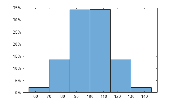
Generate 100,000 normally distributed random numbers. Use a standard deviation of 15 and a mean of 100.
x = 100 + 15*randn(1e5,1);
Plot a histogram of the random numbers. Scale and label the _y_-axis as percentages.
edges = 55:15:145; histogram(x,edges,Normalization="percentage") ytickformat("percentage")
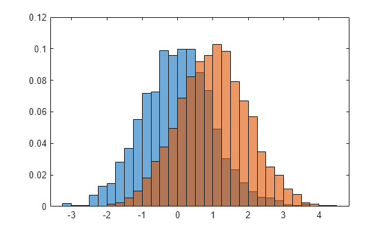
Generate two vectors of random numbers and plot a histogram for each vector in the same figure.
x = randn(2000,1); y = 1 + randn(5000,1); h1 = histogram(x); hold on h2 = histogram(y);
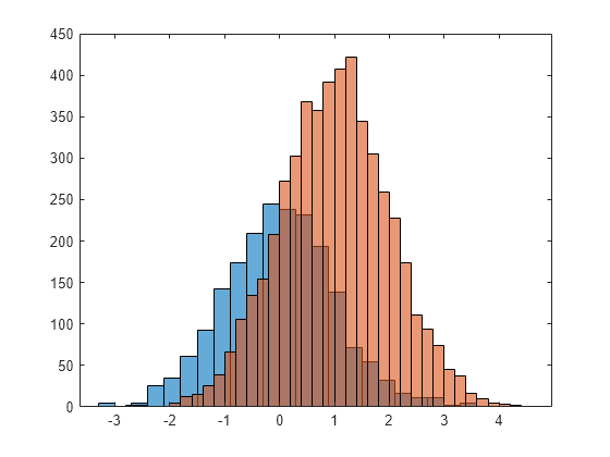
Since the sample size and bin width of the histograms are different, it is difficult to compare them. Normalize the histograms so that all of the bar heights add to 1, and use a uniform bin width.
h1.Normalization = 'probability'; h1.BinWidth = 0.25; h2.Normalization = 'probability'; h2.BinWidth = 0.25;
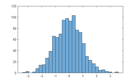
Create a histogram and return the Histogram object. Use the Histogram object to modify properties of the histogram after creating it.
x = randn(1000,1); h = histogram(x)
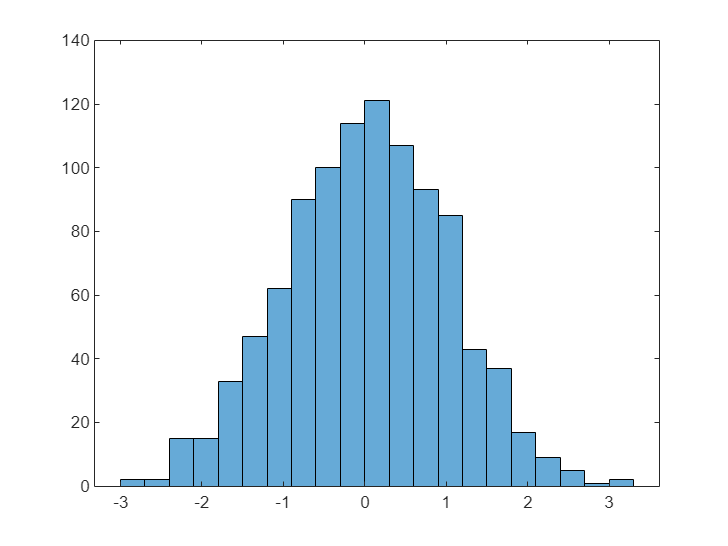
h = Histogram with properties:
         Data: [1000×1 double]
       Values: [2 2 15 15 33 47 62 90 100 114 121 107 93 85 43 37 17 9 5 1 2]
      NumBins: 21
     BinEdges: [-3.0000 -2.7000 -2.4000 -2.1000 -1.8000 -1.5000 -1.2000 -0.9000 -0.6000 -0.3000 0 0.3000 0.6000 0.9000 1.2000 1.5000 1.8000 2.1000 2.4000 2.7000 3.0000 3.3000]
     BinWidth: 0.3000
    BinLimits: [-3.0000 3.3000]
Normalization: 'count'
    FaceColor: 'auto'
    EdgeColor: [0 0 0]
Show all properties
Specify the edges of the bins with a vector.
Normalize the bin counts so that the maximum bin count is 1.
h.BinCounts = h.BinCounts/max(h.BinCounts);
You can label each rectangular bar of a histogram with the number of elements it represents.
Create a histogram.
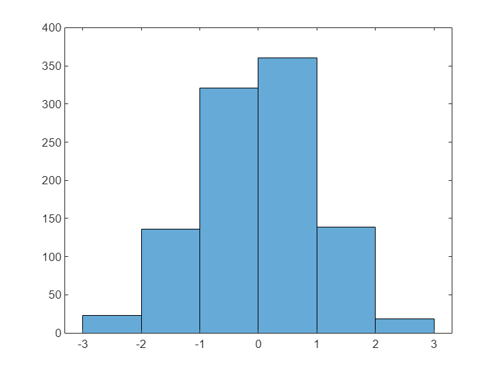
x = randn(1000,1); h = histogram(x,5);
Return the bin counts and the _x_-axis position of each bin center.
counts = h.Values; binEdges = h.BinEdges; binCenters = binEdges(1:end-1) + diff(binEdges)/2;
Add a label to each bar that displays the number of elements it represents.
text(binCenters,counts,num2str(counts'),HorizontalAlignment="center",VerticalAlignment="bottom")

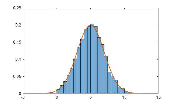
Generate 5,000 normally distributed random numbers with a mean of 5 and a standard deviation of 2. Plot a histogram with Normalization set to 'pdf' to produce an estimation of the probability density function.
x = 2*randn(5000,1) + 5; histogram(x,'Normalization','pdf')
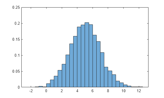
In this example, the underlying distribution for the normally distributed data is known. You can, however, use the 'pdf' histogram plot to determine the underlying probability distribution of the data by comparing it against a known probability density function.
The probability density function for a normal distribution with mean μ, standard deviation σ, and variance σ2 is
f(x,μ,σ)=1σ2π exp[-(x-μ)22σ2].
Overlay a plot of the probability density function for a normal distribution with a mean of 5 and a standard deviation of 2.
hold on y = -5:0.1:15; mu = 5; sigma = 2; f = exp(-(y-mu).^2./(2sigma^2))./(sigmasqrt(2*pi)); plot(y,f,'LineWidth',1.5)
Use the savefig function to save a histogram figure.
histogram(randn(10)); savefig('histogram.fig'); close gcf
Use openfig to load the histogram figure back into MATLAB®. openfig also returns a handle to the figure, h.
h = openfig('histogram.fig');
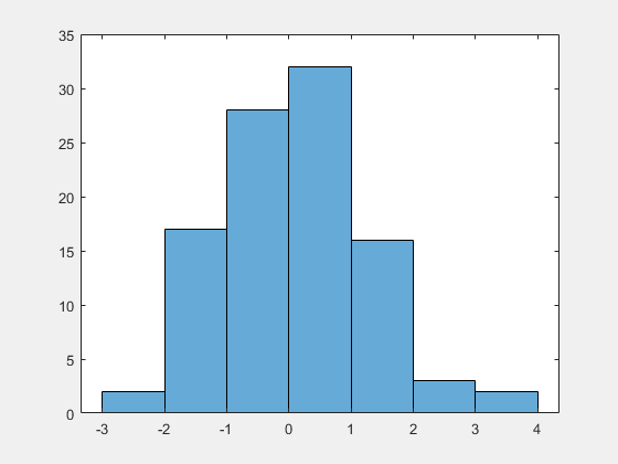
Use the findobj function to locate the correct object handle from the figure handle. This allows you to continue manipulating the original histogram object used to generate the figure.
y = findobj(h,'type','histogram')
y = Histogram with properties:
         Data: [10×10 double]
       Values: [2 17 28 32 16 3 2]
      NumBins: 7
     BinEdges: [-3 -2 -1 0 1 2 3 4]
     BinWidth: 1
    BinLimits: [-3 4]
Normalization: 'count'
    FaceColor: 'auto'
    EdgeColor: [0.1294 0.1294 0.1294]
Show all properties
Tips
- Histogram plots created using
histogramhave a context menu in plot edit mode that enables interactive manipulations in the figure window. For example, you can use the context menu to interactively change the number of bins, align multiple histograms, or change the display order. - When you add data tips to a histogram plot, they display the bin edges and bin count.
Extended Capabilities
This function supports tall arrays with the limitations:
- Some input options are not supported. The allowed options are:
'BinWidth''BinLimits''Normalization''DisplayStyle''BinMethod'— The'auto'and'scott'bin methods are the same. The'fd'bin method is not supported.'EdgeAlpha''EdgeColor''FaceAlpha''FaceColor''LineStyle''LineWidth''Orientation'
- Additionally, there is a cap on the maximum number of bars. The default maximum is 100.
- The
morebinsandfewerbinsmethods are not supported. - Editing properties of the histogram object that require recomputing the bins is not supported.
For more information, see Tall Arrays for Out-of-Memory Data.
The histogram function supports GPU array input with these usage notes and limitations:
- This function accepts GPU arrays, but does not run on a GPU.
For more information, see Run MATLAB Functions on a GPU (Parallel Computing Toolbox).
Version History
Introduced in R2014b
You can create histograms with percentages on the vertical axis by setting theNormalization name-value argument to'percentage'.