Partition Pools for Efficient Resource Management in Concurrent Parallel Workflows - MATLAB & Simulink (original) (raw)

This example shows how to use pool partitions to effectively manage and optimize resource allocation in concurrent parallel workflows.

Pool partitions allow you to execute multiple workflows simultaneously without interference, enabling precise control over resource usage for each workflow. By assigning specific computations such as parfor, parfeval, and spmd to designated pool partitions, you can ensure that each workflow operates independently and efficiently.

This method is particularly advantageous for organizing parallel pipeline workflows, where different stages can have varying resource needs. In such scenarios, pool partitions facilitate smooth data flow through the pipeline by tailoring resource allocation to match the requirements of each stage. Additionally, pool partitions are beneficial when running separate workflows concurrently, as they help manage and limit the resources each workflow consumes.

This example illustrates the use of pool partitions in executing a simulation parallel pipeline with multiple GPUs alongside a Monte Carlo path planning simulation. You can adapt this approach to manage the execution of various workflows concurrently to ensure optimal resource distribution and workflow performance.

Create Pool Partitions

Start a parallel pool with 16 workers. For this example, the myCluster profile requests a parallel pool with 16 workers from a remote cluster, where each host has eight workers and two GPUs.

pool = parpool("myCluster",16);

Starting parallel pool (parpool) using the 'myCluster' profile ... Connected to parallel pool with 16 workers.

Create pool partitions tailored to the requirements of different stages in the simulation pipeline using the partition function.

Use the partition function to create a pool partition with one worker for each available GPU for best performance. If you do not have a GPU in the pool, the gpuPool partition returns an empty parallel.pool object and the GPU computations run on the client.

[gpuPool,cpuPool] = partition(pool,"MaxNumWorkersPerGPU",1);

Using the remaining workers in the cpuPool partition, create two additional partitions. One with four workers and another with the rest of the workers in the cpuPool partition. You need at least five workers to run the simulation pipeline and parfor-loop in parallel. If you do not have enough workers, reduce the number of workers you partition for the cpuLidarPool partition.

cpuWorkers = cpuPool.Workers; [cpuLidarPool,cpuOtherPool] = partition(cpuPool,"Workers",cpuWorkers(1:4));

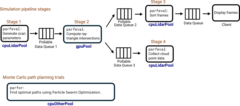
This graphic illustrates how the simulation pipeline stages and the Monte Carlo path planning trials use the pool partitions.

Perform Simulation Pipeline on Pool Partitions

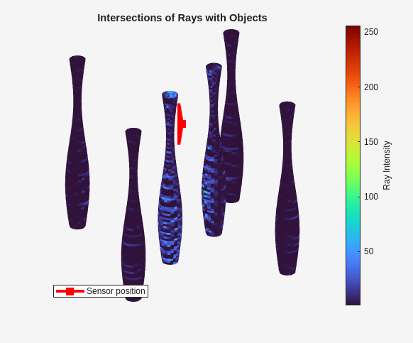
In this example, the parallel simulation pipeline models a lidar scanning system using ray tracing. Lidar sensors, similar to radar and sonar, measure distances by emitting laser pulses that reflect off objects, allowing them to perceive the structure of their surroundings. By implementing ray tracing algorithms and performing intersection calculations on multiple GPUs, you can simulate a lidar scanning system to gather information about nearby structures in a scene and generate a point cloud map of the environment.

The pipeline calculates intersections between the triangulated scene and laser rays to determine how much light hits the object surfaces. To speed up these calculations, use the Möller-Trumbore[1] algorithm, modified to run on the GPU with arrayfun.

To further enhance simulation speed, execute the simulation stages as a parallel pipeline with multiple parfeval computations. To ensure that the different stages run on the correct workers, run the parfeval computations on the gpuPool and cpuLidarPool partitions.

Stage 1: In a long-running parfeval computation, a CPU worker from the cpuLidarPool partition generates input parameters, such as the lidar sensor position and ray directions for each timestep. The worker sends these parameters to stage 2 of the pipeline using a pollable data queue. The worker also triggers a parfeval computation that performs the ray-triangle intersection calculation on the GPU.
Stage 2: Use multiple parfeval computations instead of a long-running computation. A GPU worker from the gpuPool partition runs a parfeval computation that polls a pollable data queue for data from stage 1, finds the intersections between the rays and the object surfaces, and sends the results to stages 3 and 4 using two pollable data queues.
Stage 3: A long-running parfeval computation sorts the results from stage 2 and sends them to the client in sequential order for display using a data queue.
Stage 4: Two long-running parfeval computations generate the lidar points cloud by aggregating the intersection distance results from stage 2.

Initialize Simulation Environment and Parameters

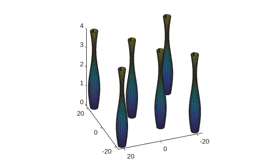
Begin by setting up a scene composed of multiple objects with triangulated surfaces. Specify the initial light position and movement parameters using the initializeParameters function, which is defined at the end of this example.

params = initializeParameters;

Next, visualize the scene using the plotScene function, also defined at the end of this example

plotScene(params); view([-110.88 31.50])

Prepare Data Queues and Define Callback Functions

To facilitate data transfer between different workers during the simulation, use a mixture of PollableDataQueue and DataQueue objects.

Create two PollableDataQueue objects with Destination set to "any" for the simulation pipeline. The first worker in the pipeline generates input parameters for each scan and sends the parameters to the stage2InputQueue pollable data queue for processing. One of the GPU workers then calculates the ray-triangle intersections and sends the results to the stage3SortQueue and stage4CloudQueue pollable data queue for further processing.

stage2InputQueue = parallel.pool.PollableDataQueue(Destination="any"); % Pollable data queue 1 stage3SortQueue = parallel.pool.PollableDataQueue(Destination="any"); % Pollable data queue 2 stage4CloudQueue = parallel.pool.PollableDataQueue(Destination="any"); % Pollable data queue 3

In this example, you run multiple, short parfeval computations on the gpuPool partition to calculate the intersections for each scan. In this way, you can interleave other parallel work on the same gpuPool partition if a worker is free. Create a DataQueue object with the name stage2TriggerQueue and use the afterEach function to define a function to run each time the stage2TriggerQueue data queue object receives data.

When the input parameters are ready, the worker running stage 1 sends a message to stage2TriggerQueue. After stage2TriggerQueue receives data, it automatically submits a parfeval computation to run the findIntersections function on the gpuPool partition. Note that the input data is already in the stage2InputQueue pollable data queue. The findIntersections function is defined at the end of the example.

stage2TriggerQueue = parallel.pool.DataQueue; afterEach(stage2TriggerQueue,@(call) ... parfeval(gpuPool,@findIntersections,0,stage2InputQueue,stage3SortQueue,stage4CloudQueue));

Prepare and initialize plots to visualize the intermediate scan data from the workers. The prepareScanningPlot function is defined at the end of this example.

[fig,s,rays] = prepareScanningPlot(params);

To track the progress of the scans on the client, create a DataQueue object with the name displayQueue. Use the afterEach function to run the displayScanFrames function when workers send data to the displayQueue data queue object. The displayScanFrames function is defined at the end of this example.

displayQueue = parallel.pool.DataQueue; afterEach(displayQueue,@(data) displayScanFrames(data,s,rays));

Start Simulation Pipeline

Stage 1 and Stage 2

For stage 1 of the pipeline, use a worker from the cpuLidarPool partition to run the addParamsToQueue function in the background with parfeval. The addParamsToQueue function continuously generates input parameters for each scan and sends them to the stage2InputQueue pollable data queue object. It also sends a message to the stage2TriggerQueue data queue object to trigger a parfeval computation on the gpuPool partition for stage 2 of the pipeline.

When the worker generates all the scan input parameters, it closes the stage2InputQueue to signal to the workers in the next stage that there is no more data to send. The addParamsToQueue function is defined at the end of this example.

fgenerate = parfeval(cpuLidarPool,@addParamsToQueue,0,params,stage2InputQueue,stage2TriggerQueue);

Stage 3

Use a worker from the cpuLidarPool partition to run the sortFrames helper function in the background with parfeval. The sortFrames function repeatedly polls the stage3SortQueue pollable data queue for new frame data, establishes a buffer for the frames, and sends them to the client in the correct sequence using the displayQueue data queue. The sortFrames function stops execution when a worker from the previous stage closes the stage3SortQueue pollable data queue. The sortFrames function is attached to this example as a supporting file.

fSort = parfeval(cpuLidarPool,@sortFrames,0,stage3SortQueue,displayQueue);

Stage 4

Run two instances of the collectCloudPointData function using workers from the cpuLidarPool partition to generate cloud point data. The collectCloudPointData function repeatedly polls the stage4CloudQueue pollable data queue for new intersection data and stops execution when a worker from the previous stage closes the stage4CloudQueue pollable data queue. The collectCloudPointData function is defined at the end of this example.

fCloud(1) = parfeval(cpuLidarPool,@collectCloudPointData,1,stage4CloudQueue); fCloud(2) = parfeval(cpuLidarPool,@collectCloudPointData,1,stage4CloudQueue);

Finally, make the figure visible to display the progress of the lidar simulation.

Perform Path Planning on Remaining Pool Partition

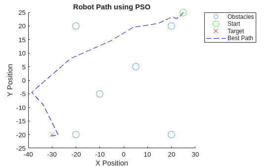
While the lidar simulation pipeline runs, you can use the remaining cpuOtherPool partition to perform additional computations. For example, you can use a parfor-loop to run multiple trials of a path planning algorithm using Particle Swarm Optimization (PSO). The goal is to find an optimal path from a starting position to a target position while avoiding objects in the scene.

Define Environment and PSO Parameters

Set up the environment parameters, including the starting and target positions, using the same scene from the simulation pipeline. Define the radius of the objects.

startPos = [25 25]; targetPos = [-30 -20]; objectRadius = ones(size(params.objectPositions,1),1)*2; obstacles = [params.objectPositions objectRadius];

Configure the parameters for the PSO algorithm, such as the number of particles, iterations, and trials. Restrict the problem to two dimensions.

numParticles = 1000; numIterations = 300; dim = 2; numTrials = 100;

Perform Path Planning Trials

Prepare to record the best path and scores for each trial. Use the parfor function to parallelize the trials for efficiency. To run the parfor-loop on the cpuOtherPool partition, specify the pool object as the second argument to the parfor function. The planPathPSO helper function is attached to this example as a supporting file.

parfor(trial = 1:numTrials,cpuOtherPool) [bestPath(trial,:,:),scores(trial)] = planPathPSO(startPos,targetPos, ... obstacles,numParticles,dim,numIterations); end

Identify the trial with the minimum score, which corresponds to the best path found by the PSO algorithm.

[~,bestInd] = min(scores);

Visualize the environment, obstacles, and the best path on a plot. The plotBestPath function is defined at the end of the example.

plotBestPath(obstacles,startPos,bestPath(bestInd,:,:),targetPos);

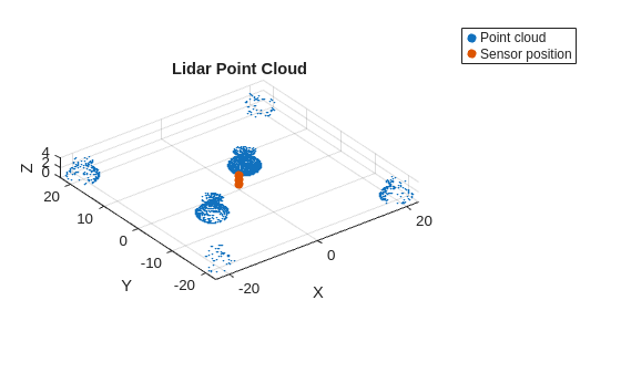
Visualize Points Cloud from Lidar Simulation

With the lidar simulation pipeline complete, you can retrieve the results from the fCloud parfeval computations.

pointCloud = fetchOutputs(fCloud);

Visualize the aggregated lidar sensor points cloud detections using the plotPointCloud function, which is defined at the end of the example. The points cloud visualizations shows the outline of the objects in the scene.

plotPointCloud(pointCloud,params);

References

[1] Möller, Tomas, and Ben Trumbore. "Fast, Minimum Storage Ray-Triangle Intersection." Journal of Graphics Tools 2, no. 1 (January 1997): 21–28. https://doi.org/10.1080/10867651.1997.10487468.

Local Supporting Functions

`addParamsToQueue` - Simulation Pipeline Stage 1

The addParamsToQueue function generates input parameters for each scan and manages their addition to a data queue for processing. For each step, it calculates the origin of the light source as it moves across the surface of the object, assigns a scan number, and sends this data to the stage2InputQueue pollable data queue. It also signals a parfeval computation to be scheduled on the GPU pool by sending a message to the stage2TriggerQueue pollable data queue. The function includes queue management to prevent the input queue from becoming overloaded by pausing when the queue length exceeds a specified threshold. After generating parameters foe all the scans, it closes the stage2InputQueue and submits a final task to the stage2TriggerQueue to close the stage 2 pollable data queues.The getScanParam helper function is attached to this example as a supporting file.

function addParamsToQueue(params,stage2InputQueue,stage2TriggerQueue) fN = 0;

numScans = size(params.lidarOrigins,1);

for scan = 1:numScans % Set lidar origin (position) lidarOrigin = params.lidarOrigins(scan,:);

for t = 1:params.totalTimeSteps
    data = getScanParam(params,t,lidarOrigin);
    fN = fN + 1;

    % Send scan number and input data to the data queue
    data.fN = fN;
    send(stage2InputQueue,data);

    % Submit parfeval computation on the GPU pool
    send(stage2TriggerQueue,"findIntersections");

    pause(0.5); % Pause to improve visualization

    % Perform some queue management to reduce strain on queue
    while stage2InputQueue.QueueLength > 10
        pause(1);
    end
end

end

% Close queue after generating all input parameters close(stage2InputQueue);

% Submit parfeval computation to close stage 2 queues send(stage2TriggerQueue,"findIntersections"); end

`findIntersections` - Simulation Pipeline Stage 2

The findIntersections function processes input parameters from a queue to calculate intersections between light rays and triangles of a 3-D object using GPU acceleration. It retrieves data from the stage2InputQueue pollable data queue and converts the ray origin and directions to gpuArray objects and uses arrayfun to perform ray-triangle intersection calculations on the GPU. It gathers the results, extracts the first intersection points and updates the data structure with the number of hits. Finally, it sends the scan number and updated data and intersection points to the stage3SortQueue and stage4CloudQueue pollable data queues respectively. The rayTriangleIntersection helper function is attached to this example as a supporting file. When no data is available in the stage2InputQueue, and poll returns OK as false because stage2InputQueue pollable data queue is closed, the function closes the stage3SortQueue and stage4CloudQueue to indicate the end of processing.

function findIntersections(stage2InputQueue,stage3SortQueue,stage4CloudQueue) [data,OK] = poll(stage2InputQueue,inf); if OK rayOriginsGPU = gpuArray(data.lidarOrigin); rayDirectionsGPU = gpuArray(data.rayDirections);

% Convert to gpuArray and calculate ray triangle intersections on the GPU
[Hits,intXs,intYs,intZs,intersectionDistances] = arrayfun(@rayTriangleIntersection, ...
    rayOriginsGPU(:,1),rayOriginsGPU(:,2),rayOriginsGPU(:,3), ...
    rayDirectionsGPU(:,1),rayDirectionsGPU(:,2),rayDirectionsGPU(:,3), ...
    data.A(:,1)',data.B(:,1)',data.C(:,1)',...
    data.A(:,2)',data.B(:,2)',data.C(:,2)', ...
    data.A(:,3)',data.B(:,3)',data.C(:,3)');

data.rayDirections = [];

% Find the closest intersection for each ray
[~,minIndices] = min(abs(intersectionDistances),[],2,"omitnan");

% Extract the first intersection points using the indices
numRays = size(intXs,1);
X = intXs(sub2ind(size(intXs),(1:numRays)',minIndices));
Y = intYs(sub2ind(size(intYs),(1:numRays)',minIndices));
Z = intZs(sub2ind(size(intZs),(1:numRays)',minIndices));

% Add intersection values to data structure
data.numHits = gather(sum(Hits,1));

% Send scan number and scan data to next worker to sort for display
output{1} = data.fN;
output{2} = data;
send(stage3SortQueue,output);

% Send intersection points to next worker
cloudData.intXs = gather(X);
cloudData.intYs = gather(Y);
cloudData.intZs = gather(Z);
send(stage4CloudQueue,cloudData);

elseif ~OK close(stage3SortQueue); close(stage4CloudQueue); end end

`collectCloudPointData` - Simulation Pipeline Stage 4

The collectCloudPointData function processes data from a the ray-intersection computation to collect and refine 3-D intersection points. It continuously polls a queue for new data, filters out invalid entries, downsamples the data, and rounds the coordinates to a specified precision. When no data is available in the stage4CloudQueue, and poll returns OK as false because a worker in the previous stage closed the stage4CloudQueue pollable data queue, the function stops execution and returns the point cloud data.

function pointCloud = collectCloudPointData(stage4CloudQueue) intersectionPoints = []; OK = true; while OK [cloudData,OK] = poll(stage4CloudQueue,inf); if ~isempty(cloudData) % Flatten the matrices X_flat = cloudData.intXs(:); Y_flat = cloudData.intYs(:); Z_flat = cloudData.intZs(:);

    % Create a logical mask for valid intersections
    validMask = ~isnan(X_flat);

    % Filter the points using the valid mask
    validX = X_flat(validMask);
    validY = Y_flat(validMask);
    validZ = Z_flat(validMask);

    % Combine the valid points into a single matrix
    thisIntersectionPoints = [validX validY validZ];
    % Downsample by selecting every nth point
    n = 5; % Downsample factor
    thisIntersectionPoints = thisIntersectionPoints(1:n:end,:);

    % Round coordinates to reduce precision
    precisionFactor = 0.01;
    thisIntersectionPoints = round(thisIntersectionPoints/precisionFactor)*precisionFactor;

    intersectionPoints = [intersectionPoints;thisIntersectionPoints];
    pointCloud = intersectionPoints;

elseif ~OK
    pointCloud = intersectionPoints;
    return
end

end end

`initializeParameters`

The initializeParameters function initializes and returns a structure containing parameters for the lidar scanning system simulation. It sets the number of rays per revolution, the number of vertical layers, the field of view of the sensor and the origin positions for the lidar scans. It also defines the surface profile for the objects in the scene and uses the createTriangulatedSurfaces helper function to generate the triangulated surface data. The createTriangulatedSurfaces helper function is attached to this example as a supporting file.

function params = initializeParameters % Define the object and create the triangulated surface params.surfProfile = 80; params.objectPositions = [-20 -20;20 -20;-20 20;20 20;-10 -5;5 5]; [params.A,params.B,params.C,params.indices] = createTriangulatedSurfaces(params.surfProfile, ... params.objectPositions);

% LiDAR Parameters params.numRaysPerRevolution = 1000; % Number of rays in one complete horizontal revolution params.numLayers = 40; % Number of vertical layers params.verticalFOV = 60; % Vertical field of view in degrees

% Simulation Parameters params.angularSpeed = 10; % Degrees per time step params.totalTimeSteps = 36; params.lidarOrigins = single([0,0,1;0,0,2;0,0,3]); % Set lidar origin (position end

`displayScanFrames`

The displayScanFrames function updates a visualization of lidar scan data by modifying the surface plot and light source based on new data.

function displayScanFrames(data,s,rays) s(1).UserData = s(1).UserData + data.numHits; indices = s(2).UserData;

% Normalize hits to range between 1 and 256 normalizedHits = rescale(s(1).UserData,1,256);

% Update surface plot with new intensities colors = repmat(normalizedHits',1,3);

for idx = 1:length(indices) rowStart = indices(idx,1); rowEnd = indices(idx,2); s(idx).CData = colors(rowStart:rowEnd,:); end

% Update origin of light source for idx = 1:size(data.rayX,1) rays(idx).XData = data.rayX(idx,:); rays(idx).YData = data.rayY(idx,:); rays(idx).ZData = data.rayZ(idx,:); end drawnow limitrate nocallbacks; end

`prepareScanningPlot`

The prepareScanningPlot function sets up a figure and axes to visualize the intersections of light rays with the object. A secondary axes plots the position of the light source as a red marker.

function [fig,s,rays] = prepareScanningPlot(params) fig = figure(Position=[933 313 582 483],Visible="off");

% Create axes for surface colors = zeros(size(params.A));

hold on for idx = 1:length(params.indices) rowStart = params.indices(idx,1); rowEnd = params.indices(idx,2); s(idx) = surf(params.A(rowStart:rowEnd,:), ... params.B(rowStart:rowEnd,:), ... params.C(rowStart:rowEnd,:), ... colors(rowStart:rowEnd,:), ... EdgeColor="none"); end hold off view([-110.88 31.50])

title("Intersections of Rays with Objects"); % Add title and axes labels axis square; axis off colormap turbo; c = colorbar; c.Label.String = "Ray Intensity"; view(160,28); s(1).UserData = zeros(1,size(params.A,1)); s(2).UserData = params.indices;

hold on for idx = 1:3 rays(idx) = plot3([NaN NaN],[NaN NaN],[NaN NaN],"r",LineWidth=3); end rays(1).MarkerIndices = 1; rays(1).Marker = "square"; rays(1).MarkerSize = 8; rays(1).MarkerFaceColor = "r"; rays(1).DisplayName = "Sensor position"; hold off axis off legend(rays(1),Location="southwest") end

`plotScene`

The plotScene function displays the scene for the lidar simulation.

function plotScene(params) figure; hold on for idx = 1:length(params.indices) rowStart = params.indices(idx,1); rowEnd = params.indices(idx,2); surf(params.A(rowStart:rowEnd,:), ... params.B(rowStart:rowEnd,:), ... params.C(rowStart:rowEnd,:)); end hold off view(3) axis square end

`plotPointCloud`

The plotPointCloud function displays the accumulated point cloud data from the lidar simulation pipeline.

function plotPointCloud(pointCloud,params) figure; scatter3(pointCloud(:,1),pointCloud(:,2),pointCloud(:,3),1,"filled"); hold on scatter3(params.lidarOrigins(:,1),params.lidarOrigins(:,2),params.lidarOrigins(:,3),"filled"); hold off xlabel("X"); ylabel("Y"); zlabel("Z"); title("Lidar Point Cloud"); legend("Point cloud","Sensor position",Location="bestoutside"); axis equal; grid on; end

`plotBestPath`

The plotBestPath function displays the environment, obstacles, and the best path from the PSO trials.

function plotBestPath(obstacles,startPos,bestPath,targetPos) figure; hold on; scatter(obstacles(:,1),obstacles(:,2),100); plot(startPos(1),startPos(2),"go","MarkerSize",10); plot(targetPos(1),targetPos(2),"rx","MarkerSize",10); plot(bestPath(1,:,1),bestPath(1,:,2),"b--"); legend("Obstacles","Start","Target","Best Path",Location="bestoutside"); title("Robot Path using PSO"); xlabel("X Position"); ylabel("Y Position"); hold off; end

Partition Pools for Efficient Resource Management in Concurrent Parallel Workflows - MATLAB & Simulink (original) (raw)

Create Pool Partitions

Perform Simulation Pipeline on Pool Partitions

Initialize Simulation Environment and Parameters

Prepare Data Queues and Define Callback Functions

Start Simulation Pipeline

Stage 1 and Stage 2

Stage 3

Stage 4

Perform Path Planning on Remaining Pool Partition

Define Environment and PSO Parameters

Perform Path Planning Trials

Visualize Points Cloud from Lidar Simulation

References

Local Supporting Functions

`addParamsToQueue` - Simulation Pipeline Stage 1

`findIntersections` - Simulation Pipeline Stage 2

`collectCloudPointData` - Simulation Pipeline Stage 4

`initializeParameters`

`displayScanFrames`

`prepareScanningPlot`

`plotScene`

`plotPointCloud`

`plotBestPath`

See Also

Topics

Partition Pools for Efficient Resource Management in Concurrent Parallel Workflows - MATLAB & Simulink (original) (raw)

Create Pool Partitions

Perform Simulation Pipeline on Pool Partitions

Initialize Simulation Environment and Parameters

Prepare Data Queues and Define Callback Functions

Start Simulation Pipeline

Stage 1 and Stage 2

Stage 3

Stage 4

Perform Path Planning on Remaining Pool Partition

Define Environment and PSO Parameters

Perform Path Planning Trials

Visualize Points Cloud from Lidar Simulation

References

Local Supporting Functions

addParamsToQueue - Simulation Pipeline Stage 1

findIntersections - Simulation Pipeline Stage 2

collectCloudPointData - Simulation Pipeline Stage 4

initializeParameters

displayScanFrames

prepareScanningPlot

plotScene

plotPointCloud

plotBestPath

See Also

Topics

`addParamsToQueue` - Simulation Pipeline Stage 1

`findIntersections` - Simulation Pipeline Stage 2

`collectCloudPointData` - Simulation Pipeline Stage 4

`initializeParameters`

`displayScanFrames`

`prepareScanningPlot`

`plotScene`

`plotPointCloud`

`plotBestPath`