margin - Classification margins for Gaussian kernel classification model - MATLAB (original) (raw)

Classification margins for Gaussian kernel classification model

Syntax

Description

[m](#d126e1281717) = margin([Mdl](#d126e1281503),[X](#d126e1281531),[Y](#mw%5F95cdc44c-0f2b-4ac5-a360-b6ff7262943f%5Fsep%5Fshared-Y)) returns the classification margins for the binary Gaussian kernel classification modelMdl using the predictor data in X and the corresponding class labels in Y.

example

[m](#d126e1281717) = margin([Mdl](#d126e1281503),[Tbl](#mw%5F95cdc44c-0f2b-4ac5-a360-b6ff7262943f%5Fsep%5Fmw%5Fc7f7abe6-14e9-4dde-ada8-1f4609c52da8),[ResponseVarName](#mw%5F95cdc44c-0f2b-4ac5-a360-b6ff7262943f%5Fsep%5Fmw%5F37cee4f7-3101-4991-b3e7-7ec414dff94d)) returns the classification margins for the trained kernel classifierMdl using the predictor data in tableTbl and the class labels inTbl.ResponseVarName.

[m](#d126e1281717) = margin([Mdl](#d126e1281503),[Tbl](#mw%5F95cdc44c-0f2b-4ac5-a360-b6ff7262943f%5Fsep%5Fmw%5Fc7f7abe6-14e9-4dde-ada8-1f4609c52da8),[Y](#mw%5F95cdc44c-0f2b-4ac5-a360-b6ff7262943f%5Fsep%5Fshared-Y)) returns the classification margins for the classifier Mdl using the predictor data in table Tbl and the class labels in vector Y.

Examples

collapse all

Load the ionosphere data set. This data set has 34 predictors and 351 binary responses for radar returns, either bad ('b') or good ('g').

Partition the data set into training and test sets. Specify a 30% holdout sample for the test set.

rng('default') % For reproducibility Partition = cvpartition(Y,'Holdout',0.30); trainingInds = training(Partition); % Indices for the training set testInds = test(Partition); % Indices for the test set

Train a binary kernel classification model using the training set.

Mdl = fitckernel(X(trainingInds,:),Y(trainingInds));

Estimate the training-set margins and test-set margins.

mTrain = margin(Mdl,X(trainingInds,:),Y(trainingInds)); mTest = margin(Mdl,X(testInds,:),Y(testInds));

Plot both sets of margins using box plots.

boxplot([mTrain; mTest],[zeros(size(mTrain,1),1); ones(size(mTest,1),1)], ... 'Labels',{'Training set','Test set'}); title('Training-Set and Test-Set Margins')

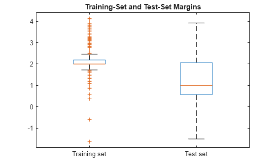
Figure contains an axes object. The axes object with title Training-Set and Test-Set Margins contains 14 objects of type line. One or more of the lines displays its values using only markers

The margin distribution of the training set is situated higher than the margin distribution of the test set.

Perform feature selection by comparing test-set margins from multiple models. Based solely on this criterion, the classifier with the larger margins is the better classifier.

Load the ionosphere data set. This data set has 34 predictors and 351 binary responses for radar returns, either bad ('b') or good ('g').

Partition the data set into training and test sets. Specify a 15% holdout sample for the test set.

rng('default') % For reproducibility Partition = cvpartition(Y,'Holdout',0.15); trainingInds = training(Partition); % Indices for the training set XTrain = X(trainingInds,:); YTrain = Y(trainingInds); testInds = test(Partition); % Indices for the test set XTest = X(testInds,:); YTest = Y(testInds);

Randomly choose 10% of the predictor variables.

p = size(X,2); % Number of predictors idxPart = randsample(p,ceil(0.1*p));

Train two binary kernel classification models: one that uses all of the predictors, and one that uses the random 10%.

Mdl = fitckernel(XTrain,YTrain); PMdl = fitckernel(XTrain(:,idxPart),YTrain);

Mdl and PMdl are ClassificationKernel models.

Estimate the test-set margins for each classifier.

fullMargins = margin(Mdl,XTest,YTest); partMargins = margin(PMdl,XTest(:,idxPart),YTest);

Plot the distribution of the margin sets using box plots.

boxplot([fullMargins partMargins], ... 'Labels',{'All Predictors','10% of the Predictors'}); title('Test-Set Margins')

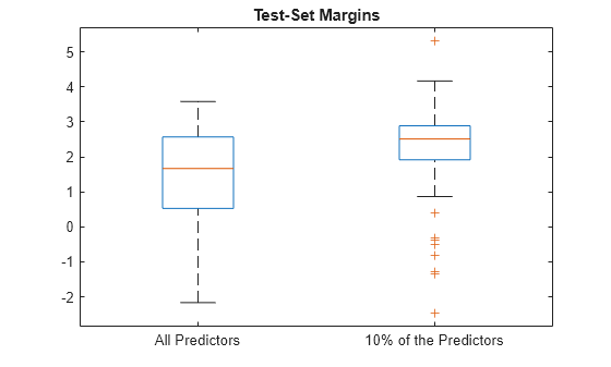
Figure contains an axes object. The axes object with title Test-Set Margins contains 14 objects of type line. One or more of the lines displays its values using only markers

The margin distribution of PMdl is situated higher than the margin distribution of Mdl. Therefore, the PMdl model is the better classifier.

Input Arguments

collapse all

Binary kernel classification model, specified as a ClassificationKernel model object. You can create aClassificationKernel model object using fitckernel.

Predictor data, specified as an n_-by-p numeric matrix, where n is the number of observations and_p is the number of predictors used to train Mdl.

The length of Y and the number of observations inX must be equal.

Data Types: single | double

Sample data used to train the model, specified as a table. Each row ofTbl corresponds to one observation, and each column corresponds to one predictor variable. Optionally, Tbl can contain additional columns for the response variable and observation weights. Tbl must contain all the predictors used to train Mdl. Multicolumn variables and cell arrays other than cell arrays of character vectors are not allowed.

If Tbl contains the response variable used to train Mdl, then you do not need to specify ResponseVarName or Y.

If you train Mdl using sample data contained in a table, then the input data for margin must also be in a table.

Response variable name, specified as the name of a variable in Tbl. If Tbl contains the response variable used to train Mdl, then you do not need to specify ResponseVarName.

If you specify ResponseVarName, then you must specify it as a character vector or string scalar. For example, if the response variable is stored asTbl.Y, then specify ResponseVarName as'Y'. Otherwise, the software treats all columns ofTbl, including Tbl.Y, as predictors.

The response variable must be a categorical, character, or string array; a logical or numeric vector; or a cell array of character vectors. If the response variable is a character array, then each element must correspond to one row of the array.

Data Types: char | string

More About

collapse all

The classification margin for binary classification is, for each observation, the difference between the classification score for the true class and the classification score for the false class.

The software defines the classification margin for binary classification as

x is an observation. If the true label of_x_ is the positive class, then y is 1, and –1 otherwise. f(x) is the positive-class classification score for the observation x. The classification margin is commonly defined as m =y f(x).

If the margins are on the same scale, then they serve as a classification confidence measure. Among multiple classifiers, those that yield greater margins are better.

For kernel classification models, the raw classification score for classifying the observation x, a row vector, into the positive class is defined by

T(·) is a transformation of an observation for feature expansion.
β is the estimated column vector of coefficients.
b is the estimated scalar bias.

The raw classification score for classifying x into the negative class is −f(x). The software classifies observations into the class that yields a positive score.

If the kernel classification model consists of logistic regression learners, then the software applies the 'logit' score transformation to the raw classification scores (see ScoreTransform).

Extended Capabilities

expand all

Themargin function supports tall arrays with the following usage notes and limitations:

margin does not support tall table data.

For more information, see Tall Arrays.

Version History

Introduced in R2017b

expand all

margin fully supports GPU arrays.