resume - Resume training of Gaussian kernel classification model - MATLAB (original) (raw)
Resume training of Gaussian kernel classification model
Syntax
Description
[UpdatedMdl](#d126e1283502) = resume([Mdl](#d126e1283029),[X](#d126e1283057),[Y](#d126e1283098)) continues training with the same options used to train Mdl, including the training data (predictor data in X and class labels in Y) and the feature expansion. The training starts at the current estimated parameters in Mdl. The function returns a new binary Gaussian kernel classification modelUpdatedMdl.
[UpdatedMdl](#d126e1283502) = resume([Mdl](#d126e1283029),[Tbl](#mw%5F1d579468-b817-4456-9c83-7eb7a4a99e6e),[ResponseVarName](#mw%5Ff3ca55d5-0a51-4ea0-9bc1-848dad7d62e0)) continues training with the predictor data in Tbl and the true class labels in Tbl.ResponseVarName.
[UpdatedMdl](#d126e1283502) = resume([Mdl](#d126e1283029),[Tbl](#mw%5F1d579468-b817-4456-9c83-7eb7a4a99e6e),[Y](#d126e1283098)) continues training with the predictor data in table Tbl and the true class labels in Y.
[UpdatedMdl](#d126e1283502) = resume(___,[Name,Value](#namevaluepairarguments)) specifies options using one or more name-value pair arguments in addition to any of the input argument combinations in previous syntaxes. For example, you can modify convergence control options, such as convergence tolerances and the maximum number of additional optimization iterations.
[[UpdatedMdl](#d126e1283502),[FitInfo](#d126e1283525)] = resume(___) also returns the fit information in the structure arrayFitInfo.
Examples
Load the ionosphere data set. This data set has 34 predictors and 351 binary responses for radar returns, either bad ('b') or good ('g').
Partition the data set into training and test sets. Specify a 20% holdout sample for the test set.
rng('default') % For reproducibility Partition = cvpartition(Y,'Holdout',0.20); trainingInds = training(Partition); % Indices for the training set XTrain = X(trainingInds,:); YTrain = Y(trainingInds); testInds = test(Partition); % Indices for the test set XTest = X(testInds,:); YTest = Y(testInds);
Train a binary kernel classification model that identifies whether the radar return is bad ('b') or good ('g').
Mdl = fitckernel(XTrain,YTrain,'IterationLimit',5,'Verbose',1);
|=================================================================================================================| | Solver | Pass | Iteration | Objective | Step | Gradient | Relative | sum(beta~=0) | | | | | | | magnitude | change in Beta | | |=================================================================================================================| | LBFGS | 1 | 0 | 1.000000e+00 | 0.000000e+00 | 2.811388e-01 | | 0 | | LBFGS | 1 | 1 | 7.585395e-01 | 4.000000e+00 | 3.594306e-01 | 1.000000e+00 | 2048 | | LBFGS | 1 | 2 | 7.160994e-01 | 1.000000e+00 | 2.028470e-01 | 6.923988e-01 | 2048 | | LBFGS | 1 | 3 | 6.825272e-01 | 1.000000e+00 | 2.846975e-02 | 2.388909e-01 | 2048 | | LBFGS | 1 | 4 | 6.699435e-01 | 1.000000e+00 | 1.779359e-02 | 1.325304e-01 | 2048 | | LBFGS | 1 | 5 | 6.535619e-01 | 1.000000e+00 | 2.669039e-01 | 4.112952e-01 | 2048 | |=================================================================================================================|
Mdl is a ClassificationKernel model.
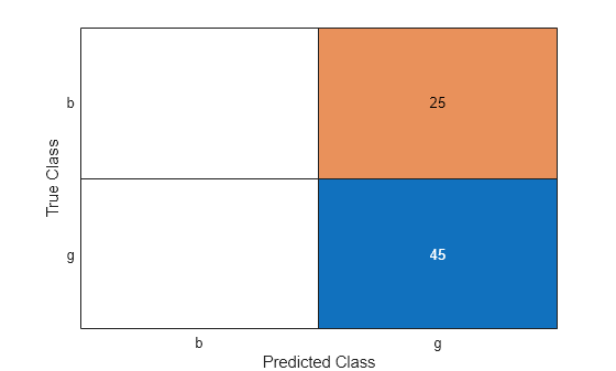
Predict the test-set labels, construct a confusion matrix for the test set, and estimate the classification error for the test set.
label = predict(Mdl,XTest); ConfusionTest = confusionchart(YTest,label);

L = loss(Mdl,XTest,YTest)
Mdl misclassifies all bad radar returns as good returns.
Continue training by using resume. This function continues training with the same options used for training Mdl.
UpdatedMdl = resume(Mdl,XTrain,YTrain);
|=================================================================================================================|
| Solver | Pass | Iteration | Objective | Step | Gradient | Relative | sum(beta=0) |
| | | | | | magnitude | change in Beta | |
|=================================================================================================================|
| LBFGS | 1 | 0 | 6.535619e-01 | 0.000000e+00 | 2.669039e-01 | | 2048 |
| LBFGS | 1 | 1 | 6.132547e-01 | 1.000000e+00 | 6.355537e-03 | 1.522092e-01 | 2048 |
| LBFGS | 1 | 2 | 5.938316e-01 | 4.000000e+00 | 3.202847e-02 | 1.498036e-01 | 2048 |
| LBFGS | 1 | 3 | 4.169274e-01 | 1.000000e+00 | 1.530249e-01 | 7.234253e-01 | 2048 |
| LBFGS | 1 | 4 | 3.679212e-01 | 5.000000e-01 | 2.740214e-01 | 2.495886e-01 | 2048 |
| LBFGS | 1 | 5 | 3.332261e-01 | 1.000000e+00 | 1.423488e-02 | 9.558680e-02 | 2048 |
| LBFGS | 1 | 6 | 3.235335e-01 | 1.000000e+00 | 7.117438e-03 | 7.137260e-02 | 2048 |
| LBFGS | 1 | 7 | 3.112331e-01 | 1.000000e+00 | 6.049822e-02 | 1.252157e-01 | 2048 |
| LBFGS | 1 | 8 | 2.972144e-01 | 1.000000e+00 | 7.117438e-03 | 5.796240e-02 | 2048 |
| LBFGS | 1 | 9 | 2.837450e-01 | 1.000000e+00 | 8.185053e-02 | 1.484733e-01 | 2048 |
| LBFGS | 1 | 10 | 2.797642e-01 | 1.000000e+00 | 3.558719e-02 | 5.856842e-02 | 2048 |
| LBFGS | 1 | 11 | 2.771280e-01 | 1.000000e+00 | 2.846975e-02 | 2.349433e-02 | 2048 |
| LBFGS | 1 | 12 | 2.741570e-01 | 1.000000e+00 | 3.914591e-02 | 3.113194e-02 | 2048 |
| LBFGS | 1 | 13 | 2.725701e-01 | 5.000000e-01 | 1.067616e-01 | 8.729821e-02 | 2048 |
| LBFGS | 1 | 14 | 2.667147e-01 | 1.000000e+00 | 3.914591e-02 | 3.491723e-02 | 2048 |
| LBFGS | 1 | 15 | 2.621152e-01 | 1.000000e+00 | 7.117438e-03 | 5.104726e-02 | 2048 |
| LBFGS | 1 | 16 | 2.601652e-01 | 1.000000e+00 | 3.558719e-02 | 3.764904e-02 | 2048 |
| LBFGS | 1 | 17 | 2.589052e-01 | 1.000000e+00 | 3.202847e-02 | 3.655744e-02 | 2048 |
| LBFGS | 1 | 18 | 2.583185e-01 | 1.000000e+00 | 7.117438e-03 | 6.490571e-02 | 2048 |
| LBFGS | 1 | 19 | 2.556482e-01 | 1.000000e+00 | 9.252669e-02 | 4.601390e-02 | 2048 |
| LBFGS | 1 | 20 | 2.542643e-01 | 1.000000e+00 | 7.117438e-02 | 4.141838e-02 | 2048 |
|=================================================================================================================|
| Solver | Pass | Iteration | Objective | Step | Gradient | Relative | sum(beta=0) |
| | | | | | magnitude | change in Beta | |
|=================================================================================================================|
| LBFGS | 1 | 21 | 2.532117e-01 | 1.000000e+00 | 1.067616e-02 | 1.661720e-02 | 2048 |
| LBFGS | 1 | 22 | 2.529890e-01 | 1.000000e+00 | 2.135231e-02 | 1.231678e-02 | 2048 |
| LBFGS | 1 | 23 | 2.523232e-01 | 1.000000e+00 | 3.202847e-02 | 1.958586e-02 | 2048 |
| LBFGS | 1 | 24 | 2.506736e-01 | 1.000000e+00 | 1.779359e-02 | 2.474613e-02 | 2048 |
| LBFGS | 1 | 25 | 2.501995e-01 | 1.000000e+00 | 1.779359e-02 | 2.514352e-02 | 2048 |
| LBFGS | 1 | 26 | 2.488242e-01 | 1.000000e+00 | 3.558719e-03 | 1.531810e-02 | 2048 |
| LBFGS | 1 | 27 | 2.485295e-01 | 5.000000e-01 | 3.202847e-02 | 1.229760e-02 | 2048 |
| LBFGS | 1 | 28 | 2.482244e-01 | 1.000000e+00 | 4.270463e-02 | 8.970983e-03 | 2048 |
| LBFGS | 1 | 29 | 2.479714e-01 | 1.000000e+00 | 3.558719e-03 | 7.393900e-03 | 2048 |
| LBFGS | 1 | 30 | 2.477316e-01 | 1.000000e+00 | 3.202847e-02 | 3.268087e-03 | 2048 |
| LBFGS | 1 | 31 | 2.476178e-01 | 2.500000e-01 | 3.202847e-02 | 5.445890e-03 | 2048 |
| LBFGS | 1 | 32 | 2.474874e-01 | 1.000000e+00 | 1.779359e-02 | 3.535903e-03 | 2048 |
| LBFGS | 1 | 33 | 2.473980e-01 | 1.000000e+00 | 7.117438e-03 | 2.821725e-03 | 2048 |
| LBFGS | 1 | 34 | 2.472935e-01 | 1.000000e+00 | 3.558719e-03 | 2.699880e-03 | 2048 |
| LBFGS | 1 | 35 | 2.471418e-01 | 1.000000e+00 | 3.558719e-03 | 1.242523e-02 | 2048 |
| LBFGS | 1 | 36 | 2.469862e-01 | 1.000000e+00 | 2.846975e-02 | 7.895605e-03 | 2048 |
| LBFGS | 1 | 37 | 2.469598e-01 | 1.000000e+00 | 2.135231e-02 | 6.657676e-03 | 2048 |
| LBFGS | 1 | 38 | 2.466941e-01 | 1.000000e+00 | 3.558719e-02 | 4.654690e-03 | 2048 |
| LBFGS | 1 | 39 | 2.466660e-01 | 5.000000e-01 | 1.423488e-02 | 2.885769e-03 | 2048 |
| LBFGS | 1 | 40 | 2.465605e-01 | 1.000000e+00 | 3.558719e-03 | 4.562565e-03 | 2048 |
|=================================================================================================================|
| Solver | Pass | Iteration | Objective | Step | Gradient | Relative | sum(beta=0) |
| | | | | | magnitude | change in Beta | |
|=================================================================================================================|
| LBFGS | 1 | 41 | 2.465362e-01 | 1.000000e+00 | 1.423488e-02 | 5.652180e-03 | 2048 |
| LBFGS | 1 | 42 | 2.463528e-01 | 1.000000e+00 | 3.558719e-03 | 2.389759e-03 | 2048 |
| LBFGS | 1 | 43 | 2.463207e-01 | 1.000000e+00 | 1.511170e-03 | 3.738286e-03 | 2048 |
| LBFGS | 1 | 44 | 2.462585e-01 | 5.000000e-01 | 7.117438e-02 | 2.321693e-03 | 2048 |
| LBFGS | 1 | 45 | 2.461742e-01 | 1.000000e+00 | 7.117438e-03 | 2.599725e-03 | 2048 |
| LBFGS | 1 | 46 | 2.461434e-01 | 1.000000e+00 | 3.202847e-02 | 3.186923e-03 | 2048 |
| LBFGS | 1 | 47 | 2.461115e-01 | 1.000000e+00 | 7.117438e-03 | 1.530711e-03 | 2048 |
| LBFGS | 1 | 48 | 2.460814e-01 | 1.000000e+00 | 1.067616e-02 | 1.811714e-03 | 2048 |
| LBFGS | 1 | 49 | 2.460533e-01 | 5.000000e-01 | 1.423488e-02 | 1.012252e-03 | 2048 |
| LBFGS | 1 | 50 | 2.460111e-01 | 1.000000e+00 | 1.423488e-02 | 4.166762e-03 | 2048 |
| LBFGS | 1 | 51 | 2.459414e-01 | 1.000000e+00 | 1.067616e-02 | 3.271946e-03 | 2048 |
| LBFGS | 1 | 52 | 2.458809e-01 | 1.000000e+00 | 1.423488e-02 | 1.846440e-03 | 2048 |
| LBFGS | 1 | 53 | 2.458479e-01 | 1.000000e+00 | 1.067616e-02 | 1.180871e-03 | 2048 |
| LBFGS | 1 | 54 | 2.458146e-01 | 1.000000e+00 | 1.455008e-03 | 1.422954e-03 | 2048 |
| LBFGS | 1 | 55 | 2.457878e-01 | 1.000000e+00 | 7.117438e-03 | 1.880892e-03 | 2048 |
| LBFGS | 1 | 56 | 2.457519e-01 | 1.000000e+00 | 2.491103e-02 | 1.074764e-03 | 2048 |
| LBFGS | 1 | 57 | 2.457420e-01 | 1.000000e+00 | 7.473310e-02 | 9.511878e-04 | 2048 |
| LBFGS | 1 | 58 | 2.457212e-01 | 1.000000e+00 | 3.558719e-03 | 3.718564e-04 | 2048 |
| LBFGS | 1 | 59 | 2.457089e-01 | 1.000000e+00 | 4.270463e-02 | 6.237270e-04 | 2048 |
| LBFGS | 1 | 60 | 2.457047e-01 | 5.000000e-01 | 1.423488e-02 | 3.647573e-04 | 2048 |
|=================================================================================================================|
| Solver | Pass | Iteration | Objective | Step | Gradient | Relative | sum(beta=0) |
| | | | | | magnitude | change in Beta | |
|=================================================================================================================|
| LBFGS | 1 | 61 | 2.456991e-01 | 1.000000e+00 | 1.423488e-02 | 5.666884e-04 | 2048 |
| LBFGS | 1 | 62 | 2.456898e-01 | 1.000000e+00 | 1.779359e-02 | 4.697056e-04 | 2048 |
| LBFGS | 1 | 63 | 2.456792e-01 | 1.000000e+00 | 1.779359e-02 | 5.984927e-04 | 2048 |
| LBFGS | 1 | 64 | 2.456603e-01 | 1.000000e+00 | 1.403782e-03 | 5.414985e-04 | 2048 |
| LBFGS | 1 | 65 | 2.456482e-01 | 1.000000e+00 | 3.558719e-03 | 6.506293e-04 | 2048 |
| LBFGS | 1 | 66 | 2.456358e-01 | 1.000000e+00 | 1.476262e-03 | 1.284139e-03 | 2048 |
| LBFGS | 1 | 67 | 2.456124e-01 | 1.000000e+00 | 3.558719e-03 | 8.636596e-04 | 2048 |
| LBFGS | 1 | 68 | 2.455980e-01 | 1.000000e+00 | 1.067616e-02 | 9.861527e-04 | 2048 |
| LBFGS | 1 | 69 | 2.455780e-01 | 1.000000e+00 | 1.067616e-02 | 5.102487e-04 | 2048 |
| LBFGS | 1 | 70 | 2.455633e-01 | 1.000000e+00 | 3.558719e-03 | 1.228077e-03 | 2048 |
| LBFGS | 1 | 71 | 2.455449e-01 | 1.000000e+00 | 1.423488e-02 | 7.864590e-04 | 2048 |
| LBFGS | 1 | 72 | 2.455261e-01 | 1.000000e+00 | 3.558719e-02 | 1.090815e-03 | 2048 |
| LBFGS | 1 | 73 | 2.455142e-01 | 1.000000e+00 | 1.067616e-02 | 1.701506e-03 | 2048 |
| LBFGS | 1 | 74 | 2.455075e-01 | 1.000000e+00 | 1.779359e-02 | 1.504577e-03 | 2048 |
| LBFGS | 1 | 75 | 2.455008e-01 | 1.000000e+00 | 3.914591e-02 | 1.144021e-03 | 2048 |
| LBFGS | 1 | 76 | 2.454943e-01 | 1.000000e+00 | 2.491103e-02 | 3.015254e-04 | 2048 |
| LBFGS | 1 | 77 | 2.454918e-01 | 5.000000e-01 | 3.202847e-02 | 9.837523e-04 | 2048 |
| LBFGS | 1 | 78 | 2.454870e-01 | 1.000000e+00 | 1.779359e-02 | 4.328953e-04 | 2048 |
| LBFGS | 1 | 79 | 2.454865e-01 | 5.000000e-01 | 3.558719e-03 | 7.126815e-04 | 2048 |
| LBFGS | 1 | 80 | 2.454775e-01 | 1.000000e+00 | 5.693950e-02 | 8.992562e-04 | 2048 |
|=================================================================================================================|
| Solver | Pass | Iteration | Objective | Step | Gradient | Relative | sum(beta=0) |
| | | | | | magnitude | change in Beta | |
|=================================================================================================================|
| LBFGS | 1 | 81 | 2.454686e-01 | 1.000000e+00 | 1.183730e-03 | 1.590246e-04 | 2048 |
| LBFGS | 1 | 82 | 2.454612e-01 | 1.000000e+00 | 2.135231e-02 | 1.389570e-04 | 2048 |
| LBFGS | 1 | 83 | 2.454506e-01 | 1.000000e+00 | 3.558719e-03 | 6.162089e-04 | 2048 |
| LBFGS | 1 | 84 | 2.454436e-01 | 1.000000e+00 | 1.423488e-02 | 1.877414e-03 | 2048 |
| LBFGS | 1 | 85 | 2.454378e-01 | 1.000000e+00 | 1.423488e-02 | 3.370852e-04 | 2048 |
| LBFGS | 1 | 86 | 2.454249e-01 | 1.000000e+00 | 1.423488e-02 | 8.133615e-04 | 2048 |
| LBFGS | 1 | 87 | 2.454101e-01 | 1.000000e+00 | 1.067616e-02 | 3.872088e-04 | 2048 |
| LBFGS | 1 | 88 | 2.453963e-01 | 1.000000e+00 | 1.779359e-02 | 5.670260e-04 | 2048 |
| LBFGS | 1 | 89 | 2.453866e-01 | 1.000000e+00 | 1.067616e-02 | 1.444984e-03 | 2048 |
| LBFGS | 1 | 90 | 2.453821e-01 | 1.000000e+00 | 7.117438e-03 | 2.457270e-03 | 2048 |
| LBFGS | 1 | 91 | 2.453790e-01 | 5.000000e-01 | 6.761566e-02 | 8.228766e-04 | 2048 |
| LBFGS | 1 | 92 | 2.453603e-01 | 1.000000e+00 | 2.135231e-02 | 1.084233e-03 | 2048 |
| LBFGS | 1 | 93 | 2.453540e-01 | 1.000000e+00 | 2.135231e-02 | 2.060005e-04 | 2048 |
| LBFGS | 1 | 94 | 2.453482e-01 | 1.000000e+00 | 1.779359e-02 | 1.560883e-04 | 2048 |
| LBFGS | 1 | 95 | 2.453461e-01 | 1.000000e+00 | 1.779359e-02 | 1.614693e-03 | 2048 |
| LBFGS | 1 | 96 | 2.453371e-01 | 1.000000e+00 | 3.558719e-02 | 2.145835e-04 | 2048 |
| LBFGS | 1 | 97 | 2.453305e-01 | 1.000000e+00 | 4.270463e-02 | 7.602088e-04 | 2048 |
| LBFGS | 1 | 98 | 2.453283e-01 | 2.500000e-01 | 2.135231e-02 | 3.422253e-04 | 2048 |
| LBFGS | 1 | 99 | 2.453246e-01 | 1.000000e+00 | 3.558719e-03 | 3.872561e-04 | 2048 |
| LBFGS | 1 | 100 | 2.453214e-01 | 1.000000e+00 | 3.202847e-02 | 1.732237e-04 | 2048 |
|=================================================================================================================|
| Solver | Pass | Iteration | Objective | Step | Gradient | Relative | sum(beta=0) |
| | | | | | magnitude | change in Beta | |
|=================================================================================================================|
| LBFGS | 1 | 101 | 2.453168e-01 | 1.000000e+00 | 1.067616e-02 | 3.065286e-04 | 2048 |
| LBFGS | 1 | 102 | 2.453155e-01 | 5.000000e-01 | 4.626335e-02 | 3.402368e-04 | 2048 |
| LBFGS | 1 | 103 | 2.453136e-01 | 1.000000e+00 | 1.779359e-02 | 2.215029e-04 | 2048 |
| LBFGS | 1 | 104 | 2.453119e-01 | 1.000000e+00 | 3.202847e-02 | 4.142355e-04 | 2048 |
| LBFGS | 1 | 105 | 2.453093e-01 | 1.000000e+00 | 1.423488e-02 | 2.186007e-04 | 2048 |
| LBFGS | 1 | 106 | 2.453090e-01 | 1.000000e+00 | 2.846975e-02 | 1.338602e-03 | 2048 |
| LBFGS | 1 | 107 | 2.453048e-01 | 1.000000e+00 | 1.423488e-02 | 3.208296e-04 | 2048 |
| LBFGS | 1 | 108 | 2.453040e-01 | 1.000000e+00 | 3.558719e-02 | 1.294488e-03 | 2048 |
| LBFGS | 1 | 109 | 2.452977e-01 | 1.000000e+00 | 1.423488e-02 | 8.328380e-04 | 2048 |
| LBFGS | 1 | 110 | 2.452934e-01 | 1.000000e+00 | 2.135231e-02 | 5.149259e-04 | 2048 |
| LBFGS | 1 | 111 | 2.452886e-01 | 1.000000e+00 | 1.779359e-02 | 3.650664e-04 | 2048 |
| LBFGS | 1 | 112 | 2.452854e-01 | 1.000000e+00 | 1.067616e-02 | 2.633981e-04 | 2048 |
| LBFGS | 1 | 113 | 2.452836e-01 | 1.000000e+00 | 1.067616e-02 | 1.804300e-04 | 2048 |
| LBFGS | 1 | 114 | 2.452817e-01 | 1.000000e+00 | 7.117438e-03 | 4.251642e-04 | 2048 |
| LBFGS | 1 | 115 | 2.452741e-01 | 1.000000e+00 | 1.779359e-02 | 9.018440e-04 | 2048 |
| LBFGS | 1 | 116 | 2.452691e-01 | 1.000000e+00 | 2.135231e-02 | 9.941716e-05 | 2048 |
|=================================================================================================================|
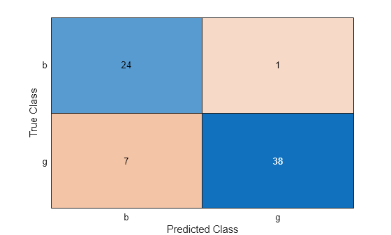
Predict the test-set labels, construct a confusion matrix for the test set, and estimate the classification error for the test set.
UpdatedLabel = predict(UpdatedMdl,XTest); UpdatedConfusionTest = confusionchart(YTest,UpdatedLabel);

UpdatedL = loss(UpdatedMdl,XTest,YTest)
The classification error decreases after resume updates the classification model with more iterations.
Load the ionosphere data set. This data set has 34 predictors and 351 binary responses for radar returns, either bad ('b') or good ('g').
Partition the data set into training and test sets. Specify a 20% holdout sample for the test set.
rng('default') % For reproducibility Partition = cvpartition(Y,'Holdout',0.20); trainingInds = training(Partition); % Indices for the training set XTrain = X(trainingInds,:); YTrain = Y(trainingInds); testInds = test(Partition); % Indices for the test set XTest = X(testInds,:); YTest = Y(testInds);
Train a binary kernel classification model with relaxed convergence control training options by using the name-value pair arguments 'BetaTolerance' and 'GradientTolerance'.
[Mdl,FitInfo] = fitckernel(XTrain,YTrain,'Verbose',1, ... 'BetaTolerance',1e-1,'GradientTolerance',1e-1);
|=================================================================================================================| | Solver | Pass | Iteration | Objective | Step | Gradient | Relative | sum(beta~=0) | | | | | | | magnitude | change in Beta | | |=================================================================================================================| | LBFGS | 1 | 0 | 1.000000e+00 | 0.000000e+00 | 2.811388e-01 | | 0 | | LBFGS | 1 | 1 | 7.585395e-01 | 4.000000e+00 | 3.594306e-01 | 1.000000e+00 | 2048 | | LBFGS | 1 | 2 | 7.160994e-01 | 1.000000e+00 | 2.028470e-01 | 6.923988e-01 | 2048 | | LBFGS | 1 | 3 | 6.825272e-01 | 1.000000e+00 | 2.846975e-02 | 2.388909e-01 | 2048 | |=================================================================================================================|
Mdl is a ClassificationKernel model.
Predict the test-set labels, construct a confusion matrix for the test set, and estimate the classification error for the test set
label = predict(Mdl,XTest); ConfusionTest = confusionchart(YTest,label);
L = loss(Mdl,XTest,YTest)
Mdl misclassifies all bad radar returns as good returns.
Continue training by using resume with modified convergence control training options.
[UpdatedMdl,UpdatedFitInfo] = resume(Mdl,XTrain,YTrain, ... 'BetaTolerance',1e-2,'GradientTolerance',1e-2);
|=================================================================================================================| | Solver | Pass | Iteration | Objective | Step | Gradient | Relative | sum(beta~=0) | | | | | | | magnitude | change in Beta | | |=================================================================================================================| | LBFGS | 1 | 0 | 6.825272e-01 | 0.000000e+00 | 2.846975e-02 | | 2048 | | LBFGS | 1 | 1 | 6.692805e-01 | 2.000000e+00 | 2.846975e-02 | 1.389258e-01 | 2048 | | LBFGS | 1 | 2 | 6.466824e-01 | 1.000000e+00 | 2.348754e-01 | 4.149425e-01 | 2048 | | LBFGS | 1 | 3 | 5.441382e-01 | 2.000000e+00 | 1.743772e-01 | 5.344538e-01 | 2048 | | LBFGS | 1 | 4 | 5.222333e-01 | 1.000000e+00 | 3.309609e-01 | 7.530878e-01 | 2048 | | LBFGS | 1 | 5 | 3.776579e-01 | 1.000000e+00 | 1.103203e-01 | 6.532621e-01 | 2048 | | LBFGS | 1 | 6 | 3.523520e-01 | 1.000000e+00 | 5.338078e-02 | 1.384232e-01 | 2048 | | LBFGS | 1 | 7 | 3.422319e-01 | 5.000000e-01 | 3.202847e-02 | 9.703897e-02 | 2048 | | LBFGS | 1 | 8 | 3.341895e-01 | 1.000000e+00 | 3.202847e-02 | 5.009485e-02 | 2048 | | LBFGS | 1 | 9 | 3.199302e-01 | 1.000000e+00 | 4.982206e-02 | 8.038014e-02 | 2048 | | LBFGS | 1 | 10 | 3.017904e-01 | 1.000000e+00 | 1.423488e-02 | 2.845012e-01 | 2048 | | LBFGS | 1 | 11 | 2.853480e-01 | 1.000000e+00 | 3.558719e-02 | 9.799137e-02 | 2048 | | LBFGS | 1 | 12 | 2.753979e-01 | 1.000000e+00 | 3.914591e-02 | 9.975305e-02 | 2048 | | LBFGS | 1 | 13 | 2.647492e-01 | 1.000000e+00 | 3.914591e-02 | 9.713710e-02 | 2048 | | LBFGS | 1 | 14 | 2.639242e-01 | 1.000000e+00 | 1.423488e-02 | 6.721803e-02 | 2048 | | LBFGS | 1 | 15 | 2.617385e-01 | 1.000000e+00 | 1.779359e-02 | 2.625089e-02 | 2048 | | LBFGS | 1 | 16 | 2.598600e-01 | 1.000000e+00 | 7.117438e-02 | 3.338724e-02 | 2048 | | LBFGS | 1 | 17 | 2.594176e-01 | 1.000000e+00 | 1.067616e-02 | 2.441171e-02 | 2048 | | LBFGS | 1 | 18 | 2.579350e-01 | 1.000000e+00 | 3.202847e-02 | 2.979246e-02 | 2048 | | LBFGS | 1 | 19 | 2.570669e-01 | 1.000000e+00 | 1.779359e-02 | 4.432998e-02 | 2048 | | LBFGS | 1 | 20 | 2.552954e-01 | 1.000000e+00 | 1.769940e-03 | 1.899895e-02 | 2048 | |=================================================================================================================|
Predict the test-set labels, construct a confusion matrix for the test set, and estimate the classification error for the test set.
UpdatedLabel = predict(UpdatedMdl,XTest); UpdatedConfusionTest = confusionchart(YTest,UpdatedLabel);
UpdatedL = loss(UpdatedMdl,XTest,YTest)
The classification error decreases after resume updates the classification model with smaller convergence tolerances.
Display the outputs FitInfo and UpdatedFitInfo.
FitInfo = struct with fields: Solver: 'LBFGS-fast' LossFunction: 'hinge' Lambda: 0.0036 BetaTolerance: 0.1000 GradientTolerance: 0.1000 ObjectiveValue: 0.6825 GradientMagnitude: 0.0285 RelativeChangeInBeta: 0.2389 FitTime: 0.0205 History: [1×1 struct]
UpdatedFitInfo = struct with fields: Solver: 'LBFGS-fast' LossFunction: 'hinge' Lambda: 0.0036 BetaTolerance: 0.0100 GradientTolerance: 0.0100 ObjectiveValue: 0.2553 GradientMagnitude: 0.0018 RelativeChangeInBeta: 0.0190 FitTime: 0.0276 History: [1×1 struct]
Both trainings terminate because the software satisfies the absolute gradient tolerance.
Plot the gradient magnitude versus the number of iterations by using UpdatedFitInfo.History.GradientMagnitude. Note that the History field of UpdatedFitInfo includes the information in the History field of FitInfo.
semilogy(UpdatedFitInfo.History.GradientMagnitude,'o-') ax = gca; ax.XTick = 1:25; ax.XTickLabel = UpdatedFitInfo.History.IterationNumber; grid on xlabel('Number of Iterations') ylabel('Gradient Magnitude')
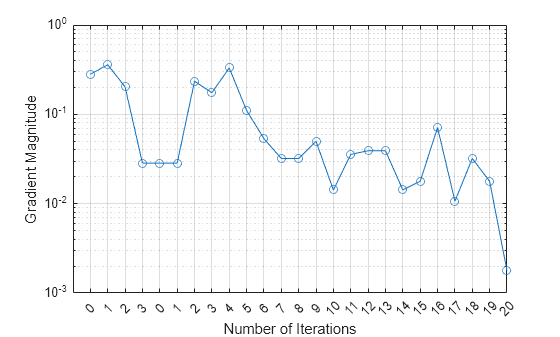
The first training terminates after three iterations because the gradient magnitude becomes less than 1e-1. The second training terminates after 20 iterations because the gradient magnitude becomes less than 1e-2.
Input Arguments
Binary kernel classification model, specified as a ClassificationKernel model object. You can create aClassificationKernel model object using fitckernel.
Predictor data used to train Mdl, specified as an_n_-by-p numeric matrix, where_n_ is the number of observations and_p_ is the number of predictors.
Data Types: single | double
Class labels used to train Mdl, specified as a categorical, character, or string array, logical or numeric vector, or cell array of character vectors.
Data Types: categorical | char | string | logical | single | double | cell
Sample data used to train Mdl, specified as a table. Each row of Tbl corresponds to one observation, and each column corresponds to one predictor variable. Optionally,Tbl can contain additional columns for the response variable and observation weights. Tbl must contain all of the predictors used to train Mdl. Multicolumn variables and cell arrays other than cell arrays of character vectors are not allowed.
If you trained Mdl using sample data contained in a table, then the input data for resume must also be in a table.
Name of the response variable used to train Mdl, specified as the name of a variable in Tbl. TheResponseVarName value must match the nameMdl.ResponseName.
Data Types: char | string
Note
resume should run only on the same training data and observation weights used to train Mdl. Theresume function uses the same training options used to train Mdl, including feature expansion.
Name-Value Arguments
Specify optional pairs of arguments asName1=Value1,...,NameN=ValueN, where Name is the argument name and Value is the corresponding value. Name-value arguments must appear after other arguments, but the order of the pairs does not matter.
Before R2021a, use commas to separate each name and value, and enclose Name in quotes.
Example: UpdatedMdl = resume(Mdl,X,Y,'GradientTolerance',1e-5) resumes training with the same options used to train Mdl, except the absolute gradient tolerance.
Observation weights used to train Mdl, specified as the comma-separated pair consisting of 'Weights' and a numeric vector or the name of a variable inTbl.
- If
Weightsis a numeric vector, then the size ofWeightsmust be equal to the number of rows in X orTbl. - If
Weightsis the name of a variable inTbl, you must specifyWeightsas a character vector or string scalar. For example, if the weights are stored asTbl.W, then specifyWeightsas'W'. Otherwise, the software treats all columns ofTbl, includingTbl.W, as predictors.
If you supply weights, resume normalizes the weights to sum up to the value of the prior probability in the respective class.
Data Types: double | single | char | string
Relative tolerance on the linear coefficients and the bias term (intercept), specified as a nonnegative scalar.
Let Bt=[βt′ bt], that is, the vector of the coefficients and the bias term at optimization iteration t. If ‖Bt−Bt−1Bt‖2<BetaTolerance, then optimization terminates.
If you also specify GradientTolerance, then optimization terminates when the software satisfies either stopping criterion.
By default, the value is the same BetaTolerance value used to train Mdl.
Example: 'BetaTolerance',1e-6
Data Types: single | double
Absolute gradient tolerance, specified as a nonnegative scalar.
Let ∇ℒt be the gradient vector of the objective function with respect to the coefficients and bias term at optimization iteration t. If ‖∇ℒt‖∞=max|∇ℒt|<GradientTolerance, then optimization terminates.
If you also specify BetaTolerance, then optimization terminates when the software satisfies either stopping criterion.
By default, the value is the same GradientTolerance value used to train Mdl.
Example: 'GradientTolerance',1e-5
Data Types: single | double
Maximum number of additional optimization iterations, specified as the comma-separated pair consisting of 'IterationLimit' and a positive integer.
The default value is 1000 if the transformed data fits in memory (Mdl.ModelParameters.BlockSize), which you specify by using the name-value pair argument when trainingMdl. Otherwise, the default value is 100.
Note that the default value is not the value used to trainMdl.
Example: 'IterationLimit',500
Data Types: single | double
Output Arguments
Optimization details, returned as a structure array including fields described in this table. The fields contain final values or name-value pair argument specifications.
| Field | Description |
|---|---|
| Solver | Objective function minimization technique:'LBFGS-fast','LBFGS-blockwise', or'LBFGS-tall'. For details, seeAlgorithms of fitckernel. |
| LossFunction | Loss function. Either 'hinge' or'logit' depending on the type of linear classification model. See Learner offitckernel. |
| Lambda | Regularization term strength. See Lambda offitckernel. |
| BetaTolerance | Relative tolerance on the linear coefficients and the bias term. See BetaTolerance. |
| GradientTolerance | Absolute gradient tolerance. SeeGradientTolerance. |
| ObjectiveValue | Value of the objective function when optimization terminates. The classification loss plus the regularization term compose the objective function. |
| GradientMagnitude | Infinite norm of the gradient vector of the objective function when optimization terminates. SeeGradientTolerance. |
| RelativeChangeInBeta | Relative changes in the linear coefficients and the bias term when optimization terminates. SeeBetaTolerance. |
| FitTime | Elapsed, wall-clock time (in seconds) required to fit the model to the data. |
| History | History of optimization information. This field also includes the optimization information from trainingMdl. This field is empty ([]) if you specify'Verbose',0 when trainingMdl. For details, see Verbose and Algorithms of fitckernel. |
To access fields, use dot notation. For example, to access the vector of objective function values for each iteration, enterFitInfo.ObjectiveValue in the Command Window.
A good practice is to examine FitInfo to assess whether convergence is satisfactory.
More About
Random feature expansion, such as Random Kitchen Sinks [1] or Fastfood [2], is a scheme to approximate Gaussian kernels of the kernel classification algorithm to use for big data in a computationally efficient way. Random feature expansion is more practical for big data applications that have large training sets, but can also be applied to smaller data sets that fit in memory.
The kernel classification algorithm searches for an optimal hyperplane that separates the data into two classes after mapping features into a high-dimensional space. Nonlinear features that are not linearly separable in a low-dimensional space can be separable in the expanded high-dimensional space. All the calculations for hyperplane classification use only dot products. You can obtain a nonlinear classification model by replacing the dot product _x_1_x_2' with the nonlinear kernel function G(x1,x2)=〈φ(x1),φ(x2)〉, where xi is the_i_th observation (row vector) and φ(xi) is a transformation that maps xi to a high-dimensional space (called the “kernel trick”). However, evaluating G(_x_1,_x_2) (Gram matrix) for each pair of observations is computationally expensive for a large data set (large n).
The random feature expansion scheme finds a random transformation so that its dot product approximates the Gaussian kernel. That is,
where T(x) maps x in ℝp to a high-dimensional space (ℝm). The Random Kitchen Sinks scheme uses the random transformation
where Z∈ℝm×p is a sample drawn from N(0,σ−2) and σ is a kernel scale. This scheme requires O(m p) computation and storage.
The Fastfood scheme introduces another random basis V instead of Z using Hadamard matrices combined with Gaussian scaling matrices. This random basis reduces the computation cost to O(mlogp) and reduces storage to O(m).
The fitckernel function uses the Fastfood scheme for random feature expansion and uses linear classification to train a Gaussian kernel classification model. Unlike solvers in the fitcsvm function, which require computation of the _n_-by-n Gram matrix, the solver in fitckernel only needs to form a matrix of size _n_-by-m, with m typically much less than n for big data.
References
[1] Rahimi, A., and B. Recht. “Random Features for Large-Scale Kernel Machines.” Advances in Neural Information Processing Systems. Vol. 20, 2008, pp. 1177–1184.
[2] Le, Q., T. Sarlós, and A. Smola. “Fastfood — Approximating Kernel Expansions in Loglinear Time.” Proceedings of the 30th International Conference on Machine Learning. Vol. 28, No. 3, 2013, pp. 244–252.
[3] Huang, P. S., H. Avron, T. N. Sainath, V. Sindhwani, and B. Ramabhadran. “Kernel methods match Deep Neural Networks on TIMIT.” 2014 IEEE International Conference on Acoustics, Speech and Signal Processing. 2014, pp. 205–209.
Extended Capabilities
Theresume function supports tall arrays with the following usage notes and limitations:
resumedoes not support talltabledata.- The default value for the
'IterationLimit'name-value pair argument is relaxed to 20 when working with tall arrays. resumeuses a block-wise strategy. For details, see Algorithms offitckernel.
For more information, see Tall Arrays.
Version History
Introduced in R2017b
resume fully supports GPU arrays.