predict - Predict labels using k-nearest neighbor classification

        model - MATLAB ([original](http://www.mathworks.com/help/stats/classificationknn.predict.html)) ([raw](?raw))

Predict labels using _k_-nearest neighbor classification model

Syntax

Description

[label](#d126e988883) = predict([mdl](#bs85nou%5Fsep%5Fshared-mdl),[X](#d126e988737)) returns a vector of predicted class labels for the predictor data in the table or matrix X, based on the trained _k_-nearest neighbor classification model mdl. See Predicted Class Label.

example

[[label](#d126e988883),[score](#d126e988927),[cost](#d126e988978)] = predict([mdl](#bs85nou%5Fsep%5Fshared-mdl),[X](#d126e988737)) also returns:

A matrix of classification scores (score) indicating the likelihood that a label comes from a particular class. For _k_-nearest neighbor, scores are posterior probabilities. See Posterior Probability.
A matrix of expected classification cost (cost). For each observation in X, the predicted class label corresponds to the minimum expected classification costs among all classes. See Expected Cost.

example

Examples

collapse all

Create a _k_-nearest neighbor classifier for Fisher's iris data, where k = 5. Evaluate some model predictions on new data.

Load the Fisher iris data set.

load fisheriris X = meas; Y = species;

Create a classifier for five nearest neighbors. Standardize the noncategorical predictor data.

mdl = fitcknn(X,Y,'NumNeighbors',5,'Standardize',1);

Predict the classifications for flowers with minimum, mean, and maximum characteristics.

Xnew = [min(X);mean(X);max(X)]; [label,score,cost] = predict(mdl,Xnew)

label = 3×1 cell {'versicolor'} {'versicolor'} {'virginica' }

score = 3×3

0.4000    0.6000         0
     0    1.0000         0
     0         0    1.0000

cost = 3×3

0.6000    0.4000    1.0000
1.0000         0    1.0000
1.0000    1.0000         0

The second and third rows of the score and cost matrices have binary values, which means all five nearest neighbors of the mean and maximum flower measurements have identical classifications.

Train _k_-nearest neighbor classifiers for various k values, and compare the decision boundaries of the classifiers.

Load the fisheriris data set.

The data set contains length and width measurements from the sepals and petals of three species of iris flowers. Remove the sepal lengths and widths, and all observed setosa irises.

inds = ~strcmp(species,'setosa'); X = meas(inds,3:4); species = species(inds);

Create a binary label variable y. The label is 1 for a virginica iris and 0 for versicolor.

y = strcmp(species,'virginica');

Train the _k-_nearest neighbor classifier. Specify 5 as the number of nearest neighbors to find, and standardize the predictor data.

EstMdl = fitcknn(X,y,'NumNeighbors',5,'Standardize',1)

EstMdl = ClassificationKNN ResponseName: 'Y' CategoricalPredictors: [] ClassNames: [0 1] ScoreTransform: 'none' NumObservations: 100 Distance: 'euclidean' NumNeighbors: 5

Properties, Methods

EstMdl is a trained ClassificationKNN classifier. Some of its properties appear in the Command Window.

Plot the decision boundary, which is the line that distinguishes between the two iris species based on their features.

x1 = min(X(:,1)):0.01:max(X(:,1)); x2 = min(X(:,2)):0.01:max(X(:,2)); [x1G,x2G] = meshgrid(x1,x2); XGrid = [x1G(:),x2G(:)]; pred = predict(EstMdl,XGrid);

figure gscatter(XGrid(:,1),XGrid(:,2),pred,[1,0,0;0,0.5,1]) hold on plot(X(y == 0,1),X(y == 0,2),'ko', ... X(y == 1,1),X(y == 1,2),'kx') xlabel('Petal length (cm)') ylabel('Petal width (cm)') title('{\bf 5-Nearest Neighbor Classifier Decision Boundary}') legend('Versicolor Region','Virginica Region', ... 'Sampled Versicolor','Sampled Virginica', ... 'Location','best') axis tight hold off

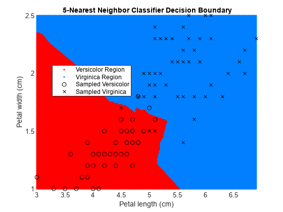
Figure contains an axes object. The axes object with title blank 5 -Nearest blank Neighbor blank Classifier blank Decision blank Boundary, xlabel Petal length (cm), ylabel Petal width (cm) contains 4 objects of type line. One or more of the lines displays its values using only markers These objects represent Versicolor Region, Virginica Region, Sampled Versicolor, Sampled Virginica.

The partition between the red and blue regions is the decision boundary. If you change the number of neighbors k, then the boundary changes.

Retrain the classifier using k = 1 (default value for NumNeighbors of fitcknn) and k = 20.

EstMdl1 = fitcknn(X,y); pred1 = predict(EstMdl1,XGrid);

EstMdl20 = fitcknn(X,y,'NumNeighbors',20); pred20 = predict(EstMdl20,XGrid);

figure gscatter(XGrid(:,1),XGrid(:,2),pred1,[1,0,0;0,0.5,1]) hold on plot(X(y == 0,1),X(y == 0,2),'ko', ... X(y == 1,1),X(y == 1,2),'kx') xlabel('Petal length (cm)') ylabel('Petal width (cm)') title('{\bf 1-Nearest Neighbor Classifier Decision Boundary}') legend('Versicolor Region','Virginica Region', ... 'Sampled Versicolor','Sampled Virginica', ... 'Location','best') axis tight hold off

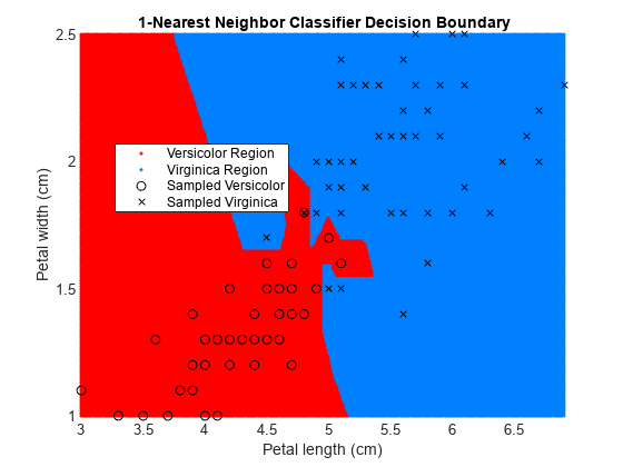
Figure contains an axes object. The axes object with title blank 1 -Nearest blank Neighbor blank Classifier blank Decision blank Boundary, xlabel Petal length (cm), ylabel Petal width (cm) contains 4 objects of type line. One or more of the lines displays its values using only markers These objects represent Versicolor Region, Virginica Region, Sampled Versicolor, Sampled Virginica.

figure gscatter(XGrid(:,1),XGrid(:,2),pred20,[1,0,0;0,0.5,1]) hold on plot(X(y == 0,1),X(y == 0,2),'ko', ... X(y == 1,1),X(y == 1,2),'kx') xlabel('Petal length (cm)') ylabel('Petal width (cm)') title('{\bf 20-Nearest Neighbor Classifier Decision Boundary}') legend('Versicolor Region','Virginica Region', ... 'Sampled Versicolor','Sampled Virginica', ... 'Location','best') axis tight hold off

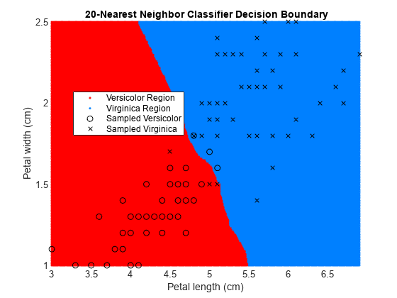
Figure contains an axes object. The axes object with title blank 20 -Nearest blank Neighbor blank Classifier blank Decision blank Boundary, xlabel Petal length (cm), ylabel Petal width (cm) contains 4 objects of type line. One or more of the lines displays its values using only markers These objects represent Versicolor Region, Virginica Region, Sampled Versicolor, Sampled Virginica.

The decision boundary seems to linearize as k increases. This linearization happens because the algorithm down-weights the importance of each input with increasing k. When k = 1, the algorithm correctly predicts the species of almost all training samples. When k = 20, the algorithm has a higher misclassification rate within the training set. You can find an optimal value of k by using the OptimizeHyperparameters name-value argument of fitcknn. For an example, see Optimize Fitted KNN Classifier.

Input Arguments

collapse all

_k_-nearest neighbor classifier model, specified as aClassificationKNN object.

Predictor data to be classified, specified as a numeric matrix or table.

Each row of X corresponds to one observation, and each column corresponds to one variable.

For a numeric matrix:
- The variables that make up the columns ofX must have the same order as the predictor variables used to trainmdl.
- If you train mdl using a table (for example, Tbl), thenX can be a numeric matrix ifTbl contains all numeric predictor variables. _k_-nearest neighbor classification requires homogeneous predictors. Therefore, to treat all numeric predictors inTbl as categorical during training, set'CategoricalPredictors','all' when you train using fitcknn. IfTbl contains heterogeneous predictors (for example, numeric and categorical data types) and X is a numeric matrix, then predict throws an error.
For a table:
- predict does not support multicolumn variables and cell arrays other than cell arrays of character vectors.
- If you train mdl using a table (for example, Tbl), then all predictor variables in X must have the same variable names and data types as those used to train mdl (stored inmdl.PredictorNames). However, the column order of X does not need to correspond to the column order ofTbl. Both Tbl andX can contain additional variables (response variables, observation weights, and so on), but predict ignores them.
- If you train mdl using a numeric matrix, then the predictor names inmdl.PredictorNames and corresponding predictor variable names inX must be the same. To specify predictor names during training, see the PredictorNames name-value pair argument of fitcknn. All predictor variables in X must be numeric vectors.X can contain additional variables (response variables, observation weights, and so on), but predict ignores them.

If you set 'Standardize',true infitcknn to train mdl, then the software standardizes the columns of X using the corresponding means in mdl.Mu and standard deviations inmdl.Sigma.

Data Types: double | single | table

Output Arguments

collapse all

Predicted class labels for the observations (rows) inX, returned as a categorical array, character array, logical vector, vector of numeric values, or cell array of character vectors. label has length equal to the number of rows in X.

For each observation, the label is the class with minimal expected cost.For an observation with NaN scores, the function classifies the observation into the majority class, which makes up the largest proportion of the training labels.

See Predicted Class Label.

Predicted class scores or posterior probabilities, returned as a numeric matrix of size _n_-by-K.n is the number of observations (rows) inX, and K is the number of classes (in mdl.ClassNames).score(i,j) is the posterior probability that observation i in X is of classj in mdl.ClassNames. See Posterior Probability.

Data Types: single | double

Expected classification costs, returned as a numeric matrix of size_n_-by-K. n is the number of observations (rows) in X, and_K_ is the number of classes (inmdl.ClassNames). cost(i,j) is the cost of classifying row i of X as class j in mdl.ClassNames. See Expected Cost.

Data Types: single | double

Algorithms

collapse all

predict classifies by minimizing the expected misclassification cost:

where:

y^ is the predicted classification.
K is the number of classes.
P^(j|x) is the posterior probability of class j for observation x.
C(y|j) is the cost of classifying an observation as y when its true class is j.

Consider a vector (single query point) xnew and a modelmdl.

k is the number of nearest neighbors used in prediction,mdl.NumNeighbors.
nbd(mdl,xnew) specifies the_k_ nearest neighbors toxnew inmdl.X.
Y(nbd) specifies the classifications of the points in nbd(mdl,xnew), namelymdl.Y(nbd).
W(nbd) specifies the weights of the points innbd(mdl,xnew).
prior specifies the priors of the classes inmdl.Y.

If the model contains a vector of prior probabilities, then the observation weightsW are normalized by class to sum to the priors. This process might involve a calculation for the point xnew, because weights can depend on the distance from xnew to the points in mdl.X.

The posterior probability p(j|xnew) is

Here, 1Y(X(i))=j is 1 whenmdl.Y(i) = j, and0 otherwise.

Two costs are associated with KNN classification: the true misclassification cost per class and the expected misclassification cost per observation.

You can set the true misclassification cost per class by using the 'Cost' name-value pair argument when you run fitcknn. The value Cost(i,j) is the cost of classifying an observation into class j if its true class is i. By default, Cost(i,j) = 1 if i ~= j, andCost(i,j) = 0 if i = j. In other words, the cost is 0 for correct classification and 1 for incorrect classification.

Two costs are associated with KNN classification: the true misclassification cost per class and the expected misclassification cost per observation. The third output of predict is the expected misclassification cost per observation.

Suppose you have Nobs observations that you want to classify with a trained classifier mdl, and you have K classes. You place the observations into a matrix Xnew with one observation per row. The command

[label,score,cost] = predict(mdl,Xnew)

returns a matrix cost of sizeNobs-by-K, among other outputs. Each row of thecost matrix contains the expected (average) cost of classifying the observation into each of the K classes. cost(n,j) is

where

K is the number of classes.
P^(i|X(n)) is the posterior probability of class i for observation Xnew(n).
C(j|i) is the true misclassification cost of classifying an observation as j when its true class is i.

Alternative Functionality

Simulink Block

To integrate the prediction of a nearest neighbor classification model into Simulink®, you can use the ClassificationKNN Predict block in the Statistics and Machine Learning Toolbox™ library or a MATLAB® Function block with the predict function. For examples, see Predict Class Labels Using ClassificationKNN Predict Block and Predict Class Labels Using MATLAB Function Block.

When deciding which approach to use, consider the following:

If you use the Statistics and Machine Learning Toolbox library block, you can use the Fixed-Point Tool (Fixed-Point Designer) to convert a floating-point model to fixed point.
Support for variable-size arrays must be enabled for a MATLAB Function block with the predict function.
If you use a MATLAB Function block, you can use MATLAB functions for preprocessing or post-processing before or after predictions in the same MATLAB Function block.

Extended Capabilities

expand all

Thepredict function fully supports tall arrays. For more information, see Tall Arrays.

Usage notes and limitations:

Use saveLearnerForCoder, loadLearnerForCoder, and codegen (MATLAB Coder) to generate code for the predict function. Save a trained model by using saveLearnerForCoder. Define an entry-point function that loads the saved model by using loadLearnerForCoder and calls thepredict function. Then use codegen to generate code for the entry-point function.
To generate single-precision C/C++ code forpredict, specify DataType="single" when you call the loadLearnerForCoder function.

This table contains notes about the arguments of predict. Arguments not included in this table are fully supported.

Argument	Notes and Limitations
mdl	AClassificationKNN model object is a full object that does not have a corresponding compact object. For this model, saveLearnerForCoder saves a compact version that does not include the hyperparameter optimization properties. If mdl is a model trained using the _k_d-tree search algorithm, and the code generation build type is a MEX function, then codegen (MATLAB Coder) generates a MEX function using Intel® Threading Building Blocks (TBB) for parallel computation. Otherwise,codegen generates code usingparfor (MATLAB Coder). MEX function for the _k_d-tree search algorithm —codegen generates an optimized MEX function using Intel TBB for parallel computation on multicore platforms. You can use the MEX function to accelerate MATLAB algorithms. For details on Intel TBB, see https://www.intel.com/content/www/us/en/developer/tools/oneapi/onetbb.html.If you generate the MEX function to test the generated code of theparfor version, you can disable the usage of Intel TBB. Set the ExtrinsicCalls property of the MEX configuration object to false. For details, see coder.MexCodeConfig (MATLAB Coder).MEX function for the exhaustive search algorithm and standalone C/C++ code for both algorithms — The generated code ofpredict uses parfor (MATLAB Coder) to create loops that run in parallel on supported shared-memory multicore platforms in the generated code. If your compiler does not support the Open Multiprocessing (OpenMP) application interface or you disable OpenMP library, MATLAB Coder™ treats the parfor-loops as for-loops. To find supported compilers, see Supported Compilers. To disable OpenMP library, set the EnableOpenMP property of the configuration object to false. For details, see coder.CodeConfig (MATLAB Coder).For the usage notes and limitations of the model object, see Code Generation of the ClassificationKNN object.
X	X must be a single-precision or double-precision matrix or a table containing numeric variables, categorical variables, or both.The number of rows, or observations, in X can be a variable size, but the number of columns in X must be fixed.If you want to specify X as a table, then your model must be trained using a table, and your entry-point function for prediction must do the following: Accept data as arrays.Create a table from the data input arguments and specify the variable names in the table.Pass the table to predict.For an example of this table workflow, see Generate Code to Classify Data in Table. For more information on using tables in code generation, see Code Generation for Tables (MATLAB Coder) and Table Limitations for Code Generation (MATLAB Coder).

Argument

Notes and Limitations

mdl

AClassificationKNN model object is a full object that does not have a corresponding compact object. For this model, saveLearnerForCoder saves a compact version that does not include the hyperparameter optimization properties. If mdl is a model trained using the _k_d-tree search algorithm, and the code generation build type is a MEX function, then codegen (MATLAB Coder) generates a MEX function using Intel® Threading Building Blocks (TBB) for parallel computation. Otherwise,codegen generates code usingparfor (MATLAB Coder). MEX function for the _k_d-tree search algorithm —codegen generates an optimized MEX function using Intel TBB for parallel computation on multicore platforms. You can use the MEX function to accelerate MATLAB algorithms. For details on Intel TBB, see https://www.intel.com/content/www/us/en/developer/tools/oneapi/onetbb.html.If you generate the MEX function to test the generated code of theparfor version, you can disable the usage of Intel TBB. Set the ExtrinsicCalls property of the MEX configuration object to false. For details, see coder.MexCodeConfig (MATLAB Coder).MEX function for the exhaustive search algorithm and standalone C/C++ code for both algorithms — The generated code ofpredict uses parfor (MATLAB Coder) to create loops that run in parallel on supported shared-memory multicore platforms in the generated code. If your compiler does not support the Open Multiprocessing (OpenMP) application interface or you disable OpenMP library, MATLAB Coder™ treats the parfor-loops as for-loops. To find supported compilers, see Supported Compilers. To disable OpenMP library, set the EnableOpenMP property of the configuration object to false. For details, see coder.CodeConfig (MATLAB Coder).For the usage notes and limitations of the model object, see Code Generation of the ClassificationKNN object.

X must be a single-precision or double-precision matrix or a table containing numeric variables, categorical variables, or both.The number of rows, or observations, in X can be a variable size, but the number of columns in X must be fixed.If you want to specify X as a table, then your model must be trained using a table, and your entry-point function for prediction must do the following: Accept data as arrays.Create a table from the data input arguments and specify the variable names in the table.Pass the table to predict.For an example of this table workflow, see Generate Code to Classify Data in Table. For more information on using tables in code generation, see Code Generation for Tables (MATLAB Coder) and Table Limitations for Code Generation (MATLAB Coder).

For more information, see Introduction to Code Generation.

Usage notes and limitations:

predict does not support GPU arrays forClassificationKNN models with the following specifications:
- The NSMethod property is specified as"kdtree".
- The Distance property is specified as"fasteuclidean", "fastseuclidean", or a function handle.
- The IncludeTies property is specified astrue.

For more information, see Run MATLAB Functions on a GPU (Parallel Computing Toolbox).

Version History

Introduced in R2012a