loss - Classification loss for neural network classifier - MATLAB (original) (raw)
Classification loss for neural network classifier
Since R2021a
Syntax
Description
`L` = loss([Mdl](#mw%5Fa68d78e6-bca5-4d72-aa1b-af5edb751c5d%5Fsep%5Fmw%5F401b4373-f245-41e6-965a-a6ce03891d5b),[Tbl](#mw%5Fa68d78e6-bca5-4d72-aa1b-af5edb751c5d%5Fsep%5Fmw%5Ff28bc064-2113-4915-ba44-719ed8f6c4ea),[ResponseVarName](#mw%5Fa68d78e6-bca5-4d72-aa1b-af5edb751c5d%5Fsep%5Fmw%5F37cee4f7-3101-4991-b3e7-7ec414dff94d)) returns the classification loss for the trained neural network classifier Mdl using the predictor data in table Tbl and the class labels in theResponseVarName table variable.
L is returned as a scalar value that represents the classification error by default.
`L` = loss([Mdl](#mw%5Fa68d78e6-bca5-4d72-aa1b-af5edb751c5d%5Fsep%5Fmw%5F401b4373-f245-41e6-965a-a6ce03891d5b),[Tbl](#mw%5Fa68d78e6-bca5-4d72-aa1b-af5edb751c5d%5Fsep%5Fmw%5Ff28bc064-2113-4915-ba44-719ed8f6c4ea),[Y](#mw%5Fa68d78e6-bca5-4d72-aa1b-af5edb751c5d%5Fsep%5Fshared-Y)) returns the classification loss for the classifier Mdl using the predictor data in table Tbl and the class labels in vectorY.
`L` = loss([Mdl](#mw%5Fa68d78e6-bca5-4d72-aa1b-af5edb751c5d%5Fsep%5Fmw%5F401b4373-f245-41e6-965a-a6ce03891d5b),[X](#mw%5Fa68d78e6-bca5-4d72-aa1b-af5edb751c5d%5Fsep%5Fmw%5F50ef4366-758a-48ab-b9a1-12ac24d79ac0),[Y](#mw%5Fa68d78e6-bca5-4d72-aa1b-af5edb751c5d%5Fsep%5Fshared-Y)) returns the classification loss for the trained neural network classifierMdl using the predictor data X and the corresponding class labels in Y.
`L` = loss(___,[Name,Value](#namevaluepairarguments)) specifies options using one or more name-value arguments in addition to any of the input argument combinations in previous syntaxes. For example, you can specify that columns in the predictor data correspond to observations, specify the loss function, or supply observation weights.
Examples
Calculate the test set classification error of a neural network classifier.
Load the patients data set. Create a table from the data set. Each row corresponds to one patient, and each column corresponds to a diagnostic variable. Use the Smoker variable as the response variable, and the rest of the variables as predictors.
load patients tbl = table(Diastolic,Systolic,Gender,Height,Weight,Age,Smoker);
Separate the data into a training set tblTrain and a test set tblTest by using a stratified holdout partition. The software reserves approximately 30% of the observations for the test data set and uses the rest of the observations for the training data set.
rng("default") % For reproducibility of the partition c = cvpartition(tbl.Smoker,"Holdout",0.30); trainingIndices = training(c); testIndices = test(c); tblTrain = tbl(trainingIndices,:); tblTest = tbl(testIndices,:);
Train a neural network classifier using the training set. Specify the Smoker column of tblTrain as the response variable. Specify to standardize the numeric predictors.
Mdl = fitcnet(tblTrain,"Smoker", ... "Standardize",true);
Calculate the test set classification error. Classification error is the default loss type for neural network classifiers.
testError = loss(Mdl,tblTest,"Smoker")
testAccuracy = 1 - testError
The neural network model correctly classifies approximately 93% of the test set observations.
Perform feature selection by comparing test set classification margins, edges, errors, and predictions. Compare the test set metrics for a model trained using all the predictors to the test set metrics for a model trained using only a subset of the predictors.
Load the sample file fisheriris.csv, which contains iris data including sepal length, sepal width, petal length, petal width, and species type. Read the file into a table.
fishertable = readtable('fisheriris.csv');
Separate the data into a training set trainTbl and a test set testTbl by using a stratified holdout partition. The software reserves approximately 30% of the observations for the test data set and uses the rest of the observations for the training data set.
rng("default") c = cvpartition(fishertable.Species,"Holdout",0.3); trainTbl = fishertable(training(c),:); testTbl = fishertable(test(c),:);
Train one neural network classifier using all the predictors in the training set, and train another classifier using all the predictors except PetalWidth. For both models, specify Species as the response variable, and standardize the predictors.
allMdl = fitcnet(trainTbl,"Species","Standardize",true); subsetMdl = fitcnet(trainTbl,"Species ~ SepalLength + SepalWidth + PetalLength", ... "Standardize",true);
Calculate the test set classification margins for the two models. Because the test set includes only 45 observations, display the margins using bar graphs.
For each observation, the classification margin is the difference between the classification score for the true class and the maximal score for the false classes. Because neural network classifiers return classification scores that are posterior probabilities, margin values close to 1 indicate confident classifications and negative margin values indicate misclassifications.
tiledlayout(2,1)
% Top axes ax1 = nexttile; allMargins = margin(allMdl,testTbl); bar(ax1,allMargins) xlabel(ax1,"Observation") ylabel(ax1,"Margin") title(ax1,"All Predictors")
% Bottom axes ax2 = nexttile; subsetMargins = margin(subsetMdl,testTbl); bar(ax2,subsetMargins) xlabel(ax2,"Observation") ylabel(ax2,"Margin") title(ax2,"Subset of Predictors")

Compare the test set classification edge, or mean of the classification margins, of the two models.
allEdge = edge(allMdl,testTbl)
subsetEdge = edge(subsetMdl,testTbl)
Based on the test set classification margins and edges, the model trained on a subset of the predictors seems to outperform the model trained on all the predictors.
Compare the test set classification error of the two models.
allError = loss(allMdl,testTbl); allAccuracy = 1-allError
subsetError = loss(subsetMdl,testTbl); subsetAccuracy = 1-subsetError
Again, the model trained using only a subset of the predictors seems to perform better than the model trained using all the predictors.
Visualize the test set classification results using confusion matrices.
allLabels = predict(allMdl,testTbl); figure confusionchart(testTbl.Species,allLabels) title("All Predictors")

subsetLabels = predict(subsetMdl,testTbl); figure confusionchart(testTbl.Species,subsetLabels) title("Subset of Predictors")

The model trained using all the predictors misclassifies four of the test set observations. The model trained using a subset of the predictors misclassifies only one of the test set observations.
Given the test set performance of the two models, consider using the model trained using all the predictors except PetalWidth.
Input Arguments
Sample data, specified as a table. Each row of Tbl corresponds to one observation, and each column corresponds to one predictor variable. Optionally, Tbl can contain an additional column for the response variable. Tbl must contain all of the predictors used to train Mdl. Multicolumn variables and cell arrays other than cell arrays of character vectors are not allowed.
- If
Tblcontains the response variable used to trainMdl, then you do not need to specify ResponseVarName or Y. - If you trained
Mdlusing sample data contained in a table, then the input data forlossmust also be in a table. - If you set
'Standardize',truein fitcnet when trainingMdl, then the software standardizes the numeric columns of the predictor data using the corresponding means and standard deviations.
Data Types: table
Response variable name, specified as the name of a variable in Tbl. If Tbl contains the response variable used to train Mdl, then you do not need to specify ResponseVarName.
If you specify ResponseVarName, then you must specify it as a character vector or string scalar. For example, if the response variable is stored asTbl.Y, then specify ResponseVarName as'Y'. Otherwise, the software treats all columns ofTbl, including Tbl.Y, as predictors.
The response variable must be a categorical, character, or string array; a logical or numeric vector; or a cell array of character vectors. If the response variable is a character array, then each element must correspond to one row of the array.
Data Types: char | string
Data Types: categorical | char | string | logical | single | double | cell
Predictor data, specified as a numeric matrix. By default,loss assumes that each row of X corresponds to one observation, and each column corresponds to one predictor variable.
Note
If you orient your predictor matrix so that observations correspond to columns and specify 'ObservationsIn','columns', then you might experience a significant reduction in computation time.
The length of Y and the number of observations in X must be equal.
If you set 'Standardize',true in fitcnet when training Mdl, then the software standardizes the numeric columns of the predictor data using the corresponding means and standard deviations.
Data Types: single | double
Name-Value Arguments
Specify optional pairs of arguments asName1=Value1,...,NameN=ValueN, where Name is the argument name and Value is the corresponding value. Name-value arguments must appear after other arguments, but the order of the pairs does not matter.
Before R2021a, use commas to separate each name and value, and enclose Name in quotes.
Example: loss(Mdl,Tbl,"Response","LossFun","crossentropy") specifies to compute the cross-entropy loss for the model Mdl.
Loss function, specified as a built-in loss function name or a function handle.
- This table lists the available loss functions. Specify one using its corresponding character vector or string scalar.
Value Description 'binodeviance' Binomial deviance 'classifcost' Observed misclassification cost 'classiferror' Misclassified rate in decimal 'crossentropy' Cross-entropy loss (for neural networks only) 'exponential' Exponential loss 'hinge' Hinge loss 'logit' Logistic loss 'mincost' Minimal expected misclassification cost (for classification scores that are posterior probabilities) 'quadratic' Quadratic loss For more details on loss functions, see Classification Loss. - To specify a custom loss function, use function handle notation. The function must have this form:
lossvalue = lossfun(C,S,W,Cost) - The output argument
lossvalueis a scalar. - You specify the function name (
lossfun). Cis ann-by-Klogical matrix with rows indicating the class to which the corresponding observation belongs.nis the number of observations in Tbl orX, andKis the number of distinct classes (numel(Mdl.ClassNames)). The column order corresponds to the class order inMdl.ClassNames. CreateCby settingC(p,q) = 1, if observationpis in classq, for each row. Set all other elements of rowpto0.Sis ann-by-Knumeric matrix of classification scores. The column order corresponds to the class order inMdl.ClassNames.Sis a matrix of classification scores, similar to the output ofpredict.Wis ann-by-1 numeric vector of observation weights.Costis aK-by-Knumeric matrix of misclassification costs. For example,Cost = ones(K) – eye(K)specifies a cost of0for correct classification and1for misclassification.
Example: 'LossFun','crossentropy'
Data Types: char | string | function_handle
Data Types: char | string
Observation weights, specified as a nonnegative numeric vector or the name of a variable in Tbl. The software weights each observation inX or Tbl with the corresponding value inWeights. The length of Weights must equal the number of observations in X orTbl.
If you specify the input data as a table Tbl, thenWeights can be the name of a variable inTbl that contains a numeric vector. In this case, you must specify Weights as a character vector or string scalar. For example, if the weights vector W is stored asTbl.W, then specify it as 'W'.
By default, Weights is ones(n,1), wheren is the number of observations in X orTbl.
If you supply weights, then loss computes the weighted classification loss and normalizes weights to sum to the value of the prior probability in the respective class.
Data Types: single | double | char | string
More About
Classification loss functions measure the predictive inaccuracy of classification models. When you compare the same type of loss among many models, a lower loss indicates a better predictive model.
Consider the following scenario.
L is the weighted average classification loss.
n is the sample size.
For binary classification:
- yj is the observed class label. The software codes it as –1 or 1, indicating the negative or positive class (or the first or second class in the
ClassNamesproperty), respectively. - f(Xj) is the positive-class classification score for observation (row) j of the predictor data X.
- mj = yj f(Xj) is the classification score for classifying observation j into the class corresponding to yj. Positive values of mj indicate correct classification and do not contribute much to the average loss. Negative values of mj indicate incorrect classification and contribute significantly to the average loss.
- yj is the observed class label. The software codes it as –1 or 1, indicating the negative or positive class (or the first or second class in the
For algorithms that support multiclass classification (that is, K ≥ 3):
- yj* is a vector of K – 1 zeros, with 1 in the position corresponding to the true, observed class_yj_. For example, if the true class of the second observation is the third class and K = 4, then _y_2* = [
0 0 1 0]′. The order of the classes corresponds to the order in theClassNamesproperty of the input model. - f(Xj) is the length K vector of class scores for observation_j_ of the predictor data X. The order of the scores corresponds to the order of the classes in the
ClassNamesproperty of the input model. - mj =yj*′f(Xj). Therefore,mj is the scalar classification score that the model predicts for the true, observed class.
- yj* is a vector of K – 1 zeros, with 1 in the position corresponding to the true, observed class_yj_. For example, if the true class of the second observation is the third class and K = 4, then _y_2* = [
The weight for observation j is_wj_. The software normalizes the observation weights so that they sum to the corresponding prior class probability stored in the
Priorproperty. Therefore,
Given this scenario, the following table describes the supported loss functions that you can specify by using the LossFun name-value argument.
| Loss Function | Value of LossFun | Equation |
|---|---|---|
| Binomial deviance | "binodeviance" | L=∑j=1nwjlog{1+exp[−2mj]}. |
| Observed misclassification cost | "classifcost" | L=∑j=1nwjcyjy^j,where y^j is the class label corresponding to the class with the maximal score, and cyjy^j is the user-specified cost of classifying an observation into class y^j when its true class is_yj_. |
| Misclassified rate in decimal | "classiferror" | L=∑j=1nwjI{y^j≠yj},where_I_{·} is the indicator function. |
| Cross-entropy loss | "crossentropy" | "crossentropy" is appropriate only for neural network models.The weighted cross-entropy loss is L=−∑j=1nw˜jlog(mj)Kn,where the weights w˜j are normalized to sum to n instead of 1. |
| Exponential loss | "exponential" | L=∑j=1nwjexp(−mj). |
| Hinge loss | "hinge" | L=∑j=1nwjmax{0,1−mj}. |
| Logistic loss | "logit" | L=∑j=1nwjlog(1+exp(−mj)). |
| Minimal expected misclassification cost | "mincost" | "mincost" is appropriate only if classification scores are posterior probabilities.The software computes the weighted minimal expected classification cost using this procedure for observations_j_ = 1,...,n. Estimate the expected misclassification cost of classifying the observation_Xj_ into the class k: γjk=(f(Xj)′C)k.f(Xj) is the column vector of class posterior probabilities for the observation_Xj_.C is the cost matrix stored in theCost property of the model.For observation j, predict the class label corresponding to the minimal expected misclassification cost: y^j=argmink=1,...,Kγjk.Using C, identify the cost incurred (cj) for making the prediction. The weighted average of the minimal expected misclassification cost loss is L=∑j=1nwjcj. |
| Quadratic loss | "quadratic" | L=∑j=1nwj(1−mj)2. |
If you use the default cost matrix (whose element value is 0 for correct classification and 1 for incorrect classification), then the loss values for"classifcost", "classiferror", and"mincost" are identical. For a model with a nondefault cost matrix, the "classifcost" loss is equivalent to the "mincost" loss most of the time. These losses can be different if prediction into the class with maximal posterior probability is different from prediction into the class with minimal expected cost. Note that "mincost" is appropriate only if classification scores are posterior probabilities.
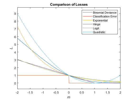
This figure compares the loss functions (except "classifcost","crossentropy", and "mincost") over the score_m_ for one observation. Some functions are normalized to pass through the point (0,1).
Extended Capabilities
Version History
Introduced in R2021a
loss fully supports GPU arrays.
Starting in R2022a, the loss function uses the"mincost" option (minimal expected misclassification cost) as the default value for the LossFun name-value argument. The"mincost" option is appropriate when classification scores are posterior probabilities. In previous releases, the default value was"classiferror".
You do not need to make any changes to your code for the default cost matrix (whose element value is 0 for correct classification and 1 for incorrect classification).
The loss function no longer omits an observation with a NaN score when computing the weighted average classification loss. Therefore,loss can now return NaN when the predictor dataX or the predictor variables in Tbl contain any missing values, and the name-value argument LossFun is not specified as "classifcost", "classiferror", or"mincost". In most cases, if the test set observations do not contain missing predictors, the loss function does not return NaN.
This change improves the automatic selection of a classification model when you usefitcauto. Before this change, the software might select a model (expected to best classify new data) with few non-NaN predictors.
If loss in your code returns NaN, you can update your code to avoid this result by doing one of the following:
- Remove or replace the missing values by using rmmissing or fillmissing, respectively.
- Specify the name-value argument
LossFunas"classifcost","classiferror", or"mincost".
The following table shows the classification models for which theloss object function might return NaN. For more details, see the Compatibility Considerations for each loss function.