predict - Predict response of linear mixed-effects model - MATLAB (original) (raw)
Predict response of linear mixed-effects model
Syntax
Description
[ypred](#btvrlby-ypred) = predict([lme](#btvrlby%5Fsep%5Fshared-lme),[tblnew](#btvrlby%5Fsep%5Fshared-tblnew)) returns a vector of conditional predicted responses ypred from the fitted linear mixed-effects model lme at the values in the new table or dataset array tblnew. Use a table or dataset array for predict if you use a table or dataset array for fitting the model lme.
If a particular grouping variable in tblnew has levels that are not in the original data, then the random effects for that grouping variable do not contribute to the 'Conditional' prediction at observations where the grouping variable has new levels.
[ypred](#btvrlby-ypred) = predict([lme](#btvrlby%5Fsep%5Fshared-lme),[Xnew](#btvrlby%5Fsep%5Fshared-Xnew),[Znew](#btvrlby%5Fsep%5Fshared-Znew)) returns a vector of conditional predicted responses ypred from the fitted linear mixed-effects model lme at the values in the new fixed- and random-effects design matrices, Xnew and Znew, respectively. Znew can also be a cell array of matrices. In this case, the grouping variable G is ones(n,1), where n is the number of observations used in the fit.
Use the matrix format for predict if using design matrices for fitting the model lme.
[ypred](#btvrlby-ypred) = predict([lme](#btvrlby%5Fsep%5Fshared-lme),[Xnew](#btvrlby%5Fsep%5Fshared-Xnew),[Znew](#btvrlby%5Fsep%5Fshared-Znew),[Gnew](#shared-Gnew)) returns a vector of conditional predicted responses ypred from the fitted linear mixed-effects model lme at the values in the new fixed- and random-effects design matrices, Xnew and Znew, respectively, and the grouping variable Gnew.
Znew and Gnew can also be cell arrays of matrices and grouping variables, respectively.
[ypred](#btvrlby-ypred) = predict(___,[Name,Value](#namevaluepairarguments)) returns a vector of predicted responses ypred from the fitted linear mixed-effects model lme with additional options specified by one or more Name,Value pair arguments.
For example, you can specify the confidence level, simultaneous confidence bounds, or contributions from only fixed effects.
[[ypred](#btvrlby-ypred),[ypredCI](#btvrlby-ypredCI)] = predict(___) also returns confidence intervals ypredCI for the predictions ypred for any of the input arguments in the previous syntaxes.
[[ypred](#btvrlby-ypred),[ypredCI](#btvrlby-ypredCI),[DF](#btvrlby-DF)] = predict(___) also returns the degrees of freedom DF used in computing the confidence intervals for any of the input arguments in the previous syntaxes.
Examples
Load the sample data.
The table tbl array includes data from a split-plot experiment, where soil is divided into three blocks based on the soil type: sandy, silty, and loamy. Each block is divided into five plots, where five different types of tomato plants (cherry, heirloom, grape, vine, and plum) are randomly assigned to these plots. The tomato plants in the plots are then divided into subplots, where each subplot is treated by one of four fertilizers. This is simulated data.
Convert the table variables Tomato, Soil, and Fertilizer to categorical variables.
tbl.Tomato = categorical(tbl.Tomato); tbl.Soil = categorical(tbl.Soil); tbl.Fertilizer = categorical(tbl.Fertilizer);
Fit a linear mixed-effects model, where Fertilizer and Tomato are the fixed-effects variables, and the mean yield varies by the block (soil type), and the plots within blocks (tomato types within soil types) independently.
lme = fitlme(tbl,'Yield ~ Fertilizer * Tomato + (1|Soil) + (1|Soil:Tomato)');
Predict the response values at the original design values. Display the first five predictions with the observed response values.
yhat = predict(lme); [yhat(1:5) tbl.Yield(1:5)]
ans = 5×2
115.4788 104.0000 135.1455 136.0000 152.8121 158.0000 160.4788 174.0000 58.0839 57.0000
Load the sample data.
Fit a linear mixed-effects model, with a fixed effect for Weight, and a random intercept grouped by Model_Year. First, store the data in a table.
tbl = table(MPG,Weight,Model_Year); lme = fitlme(tbl,'MPG ~ Weight + (1|Model_Year)');
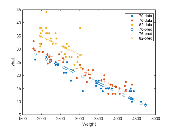
Create predicted responses to the data.
Plot the original responses and the predicted responses to see how they differ. Group them by model year.
figure() gscatter(Weight,MPG,Model_Year) hold on gscatter(Weight,yhat,Model_Year,[],'o+x') legend('70-data','76-data','82-data','70-pred','76-pred','82-pred') hold off
Load the sample data and display the variable tbl.
tbl=60×4 table Soil Tomato Fertilizer Yield _________ ____________ __________ _____
{'Sandy'}    {'Plum'    }        1          104
{'Sandy'}    {'Plum'    }        2          136
{'Sandy'}    {'Plum'    }        3          158
{'Sandy'}    {'Plum'    }        4          174
{'Sandy'}    {'Cherry'  }        1           57
{'Sandy'}    {'Cherry'  }        2           86
{'Sandy'}    {'Cherry'  }        3           89
{'Sandy'}    {'Cherry'  }        4           98
{'Sandy'}    {'Heirloom'}        1           65
{'Sandy'}    {'Heirloom'}        2           62
{'Sandy'}    {'Heirloom'}        3          113
{'Sandy'}    {'Heirloom'}        4           84
{'Sandy'}    {'Grape'   }        1           54
{'Sandy'}    {'Grape'   }        2           86
{'Sandy'}    {'Grape'   }        3           89
{'Sandy'}    {'Grape'   }        4          115
  ⋮
The table tbl includes data from a split-plot experiment, where soil is divided into three blocks based on the soil type: sandy, silty, and loamy. Each block is divided into five plots, where five different types of tomato plants (cherry, heirloom, grape, vine, and plum) are randomly assigned to these plots. The tomato plants in the plots are then divided into subplots, where each subplot is treated by one of four fertilizers. This is simulated data.
Convert the table variables Tomato, Soil, and Fertilizer as categorical variables.
tbl.Tomato = categorical(tbl.Tomato); tbl.Soil = categorical(tbl.Soil); tbl.Fertilizer = categorical(tbl.Fertilizer);
Fit a linear mixed-effects model, where Fertilizer and Tomato are the fixed-effects variables, and the mean yield varies by the block (soil type), and the plots within blocks (tomato types within soil types) independently.
lme = fitlme(tbl,"Yield ~ Fertilizer * Tomato + (1|Soil) + (1|Soil:Tomato)");
Create a new table with design values. The new dataset array must have the same variables as the original dataset array you use for fitting the model lme.
tblnew = table(); tblnew.Soil = categorical(["Sandy";"Silty"]); tblnew.Tomato = categorical(["Cherry";"Vine"]); tblnew. Fertilizer = categorical([2;2]);
Predict the conditional and marginal responses at the original design points.
yhatC = predict(lme,tblnew); yhatM = predict(lme,tblnew,Conditional=false); [yhatC yhatM]
ans = 2×2
92.7505 111.6667 87.5891 82.6667
Load the sample data.
Fit a linear mixed-effects model for miles per gallon (MPG), with fixed effects for acceleration, horsepower, and cylinders, and potentially correlated random effects for intercept and acceleration grouped by model year.
First, prepare the design matrices for fitting the linear mixed-effects model.
X = [ones(406,1) Acceleration Horsepower]; Z = [ones(406,1) Acceleration]; Model_Year = nominal(Model_Year); G = Model_Year;
Now, fit the model using fitlmematrix with the defined design matrices and grouping variables.
lme = fitlmematrix(X,MPG,Z,G,'FixedEffectPredictors',.... {'Intercept','Acceleration','Horsepower'},'RandomEffectPredictors',... {{'Intercept','Acceleration'}},'RandomEffectGroups',{'Model_Year'});
Create the design matrices that contain the data at which to predict the response values. Xnew must have three columns as in X. The first column must be a column of 1s. And the values in the last two columns must correspond to Acceleration and Horsepower, respectively. The first column of Znew must be a column of 1s, and the second column must contain the same Acceleration values as in Xnew. The original grouping variable in G is the model year. So, Gnew must contain values for the model year. Note that Gnew must contain nominal values.
Xnew = [1,13.5,185; 1,17,205; 1,21.2,193]; Znew = [1,13.5; 1,17; 1,21.2]; % alternatively Znew = Xnew(:,1:2); Gnew = nominal([73 77 82]);
Predict the responses for the data in the new design matrices.
yhat = predict(lme,Xnew,Znew,Gnew)
yhat = 3×1
8.7063
5.4423
12.5384
Now, repeat the same for a linear mixed-effects model with uncorrelated random-effects terms for intercept and acceleration. First, change the original random effects design and the random effects grouping variables. Then, refit the model.
Z = {ones(406,1),Acceleration}; G = {Model_Year,Model_Year};
lme = fitlmematrix(X,MPG,Z,G,'FixedEffectPredictors',.... {'Intercept','Acceleration','Horsepower'},'RandomEffectPredictors',... {{'Intercept'},{'Acceleration'}},'RandomEffectGroups',{'Model_Year','Model_Year'});
Now, recreate the new random effects design, Znew, and the grouping variable design, Gnew, using which to predict the response values.
Znew = {[1;1;1],[13.5;17;21.2]}; MY = nominal([73 77 82]); Gnew = {MY,MY};
Predict the responses using the new design matrices.
yhat = predict(lme,Xnew,Znew,Gnew)
yhat = 3×1
8.6365
5.9199
12.1247
Load the sample data.
Fit a linear mixed-effects model for miles per gallon (MPG), with fixed effects for acceleration, horsepower, and cylinders, and potentially correlated random effects for intercept and acceleration grouped by model year. First, store the variables in a table.
tbl = table(MPG,Acceleration,Horsepower,Model_Year);
Now, fit the model using fitlme with the defined design matrices and grouping variables.
lme = fitlme(tbl,'MPG ~ Acceleration + Horsepower + (Acceleration|Model_Year)');
Create the new data and store it in a new table.
tblnew = table(); tblnew.Acceleration = linspace(8,25)'; tblnew.Horsepower = linspace(min(Horsepower),max(Horsepower))'; tblnew.Model_Year = repmat(70,100,1);
linspace creates 100 equally distanced values between the lower and the upper input limits. Model_Year is fixed at 70. You can repeat this for any model year.
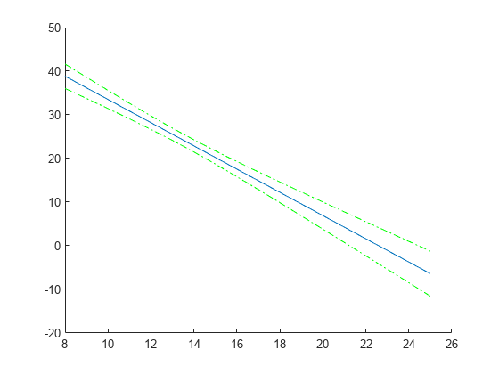
Compute and plot the predicted values and 95% confidence limits (nonsimultaneous).
[ypred,yCI,DF] = predict(lme,tblnew); figure(); h1 = line(tblnew.Acceleration,ypred); hold on; h2 = plot(tblnew.Acceleration,yCI,'g-.');
Display the degrees of freedom.
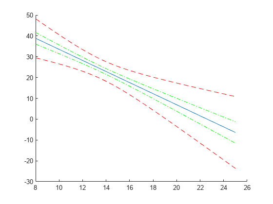
Compute and plot the simultaneous confidence bounds.
[ypred,yCI,DF] = predict(lme,tblnew,'Simultaneous',true); h3 = plot(tblnew.Acceleration,yCI,'r--');
Display the degrees of freedom.
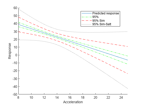
Compute the simultaneous confidence bounds using the Satterthwaite method to compute the degrees of freedom.
[ypred,yCI,DF] = predict(lme,tblnew,'Simultaneous',true,'DFMethod','satterthwaite'); h4 = plot(tblnew.Acceleration,yCI,'k:'); hold off xlabel('Acceleration') ylabel('Response') ylim([-50,60]) xlim([8,25]) legend([h1,h2(1),h3(1),h4(1)],'Predicted response','95%','95% Sim',... '95% Sim-Satt','Location','Best')
Display the degrees of freedom.
Input Arguments
New input data, which includes the response variable, predictor variables, and grouping variables, specified as a table or dataset array. The predictor variables can be continuous or grouping variables. tblnew must have the same variables as in the original table or dataset array used to fit the linear mixed-effects model lme.
New fixed-effects design matrix, specified as an _n_-by-p matrix, where n is the number of observations and p is the number of fixed predictor variables. Each row of X corresponds to one observation and each column of X corresponds to one variable.
Data Types: single | double
New random-effects design, specified as an _n_-by-q matrix or a cell array of R design matrices Z{r}, where r = 1, 2, ..., R. If Znew is a cell array, then each Z{r} is an _n_-by-q(r) matrix, where n is the number of observations, and q(r) is the number of random predictor variables.
Data Types: single | double | cell
New grouping variable or variables, specified as a vector or a cell array, of length R, of grouping variables with the same levels or groups as the original grouping variables used to fit the linear mixed-effects model lme.
Data Types: single | double | categorical | logical | char | string | cell
Name-Value Arguments
Specify optional pairs of arguments asName1=Value1,...,NameN=ValueN, where Name is the argument name and Value is the corresponding value. Name-value arguments must appear after other arguments, but the order of the pairs does not matter.
Before R2021a, use commas to separate each name and value, and enclose Name in quotes.
Example: ypred = predict(lme,'Conditional',false);
Data Types: single | double
Indicator for conditional predictions, specified as the comma-separated pair consisting of 'Conditional' and one of the following.
| true | Contributions from both fixed effects and random effects (conditional) |
|---|---|
| false | Contribution from only fixed effects (marginal) |
Example: 'Conditional,false
Method for computing approximate degrees of freedom to use in the confidence interval computation, specified as the comma-separated pair consisting of 'DFMethod' and one of the following.
| "residual" | Default. The degrees of freedom are assumed to be constant and equal to n – p, where n is the number of observations and p is the number of fixed effects. |
|---|---|
| "satterthwaite" | Satterthwaite approximation. |
| "none" | All degrees of freedom are set to infinity. |
For example, you can specify the Satterthwaite approximation as follows.
Example: 'DFMethod','satterthwaite'
Type of confidence bounds, specified as the comma-separated pair consisting of 'Simultaneous' and one of the following.
| false | Default. Nonsimultaneous bounds. |
|---|---|
| true | Simultaneous bounds. |
Example: 'Simultaneous',true
Type of prediction, specified as the comma-separated pair consisting of 'Prediction' and one of the following.
| 'curve' | Default. Confidence bounds for the predictions based on the fitted function. |
|---|---|
| 'observation' | Variability due to observation error for the new observations is also included in the confidence bound calculations and this results in wider bounds. |
Example: 'Prediction','observation'
Output Arguments
Predicted responses, returned as a vector. ypred can contain the conditional or marginal responses, depending on the value choice of the 'Conditional' name-value pair argument. Conditional predictions include contributions from both fixed and random effects.
Point-wise confidence intervals for the predicted values, returned as a two-column matrix. The first column of yCI contains the lower bounds, and the second column contains the upper bound. By default, yCI contains the 95% confidence intervals for the predictions. You can change the confidence level using the Alpha name-value pair argument, make them simultaneous using the Simultaneous name-value pair argument, and also make them for a new observation rather than for the curve using the Prediction name-value pair argument.
Degrees of freedom used in computing the confidence intervals, returned as a vector or a scalar value.
- If the 'Simultaneous' name-value pair argument is
false, thenDFis a vector. - If the
'Simultaneous'name-value pair argument istrue, thenDFis a scalar value.
More About
A conditional prediction includes contributions from both fixed and random effects, whereas a marginal model includes contribution from only fixed effects.
Suppose the linear mixed-effects model lme has an _n_-by-p fixed-effects design matrix X and an _n_-by-q random-effects design matrix Z. Also, suppose the estimated _p_-by-1 fixed-effects vector is β^, and the _q_-by-1 estimated best linear unbiased predictor (BLUP) vector of random effects is b^. The predicted conditional response is
which corresponds to the 'Conditional','true' name-value pair argument.
The predicted marginal response is
which corresponds to the 'Conditional','false' name-value pair argument.
When making predictions, if a particular grouping variable has new levels (1s that were not in the original data), then the random effects for the grouping variable do not contribute to the 'Conditional' prediction at observations where the grouping variable has new levels.
Version History
Introduced in R2013b