Pulsed Fiber Amplifier Modeling With the Software RP Fiber Power (original) (raw)

RP Fiber Power logo

RP Fiber Power — Simulation and Design Software for Fiber Optics, Amplifiers and Fiber Lasers

Power Form: Fiber Amplifier for Ultrashort Pulses

This Power Form allows one to set up sophisticated physical models for fiber amplifiers (multiple input signals, multiple stages, etc.) applied to ultrashort pulses. Here, we need to consider nonlinear and dispersive effects — in contrast to a simpler model for longer pulses where chromatic dispersion and nonlinearities can be neglected.

graphic for this Power Form

Demo Video

One of our case studies has been produced using the Power Form described here:

Your browser does not support the video tag. However, you can download the video file.

Basic features of the model

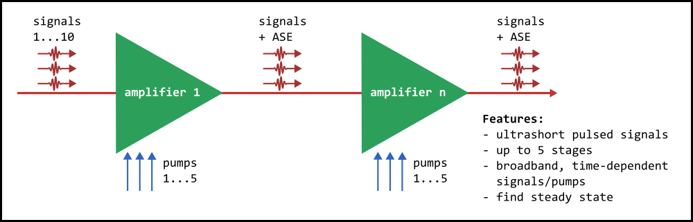
Amplifier stages: We simulate a fiber amplifier with up to five different stages. Each stage may be activated or deactivated.
Input signals: we start with up to ten input signal pulses, each of which is an ultrashort pulse, which may be specified in different ways, e.g. with some energy, duration, temporal shape and chirp.
Fiber parameters: for each amplifier stage, one can select a fiber parameter set - from a commercially available fiber, for example. One can also override various parameters.
Pump sources: each amplifier stage can have up to 5 quasi-monochromatic or broadband forward or backward pump inputs. It is assumed that no pump light can ever get from one amplifier stage to another stage.
Single or double pass amplification: normally, the signal light would get from the signal source through some number of amplifier stages, each one passing in just one direction (called forward direction). However, one can have a wavelength-dependent reflector at the end of a stage to realize a double-pass amplifier stage; in that case, the signal is propagating back through the same fiber and then separated from the input with a Faraday circulator before being sent to the next stage.
Coupling losses: after each amplifier stage, and after the input signal source, we can introduce coupling losses, which can be wavelength-dependent.
Amplified spontaneous emission (ASE) can also be considered. See the encyclopedia article on ASE. ASE may get from one stage to the next one, suffering the above-mentioned wavelength-dependent losses (e.g. from a bandpass filter), but it is assumed that it cannot get to the previous stage (e.g. due to a Faraday isolator preventing that).
Simulation cycles: we can simulate either a single pulse amplification or repetitive operation, where we also monitor how various properties evolve over multiple (possible many) pumping/amplification cycles.

Note that for cases where nonlinear and chromatic dispersion effects can be neglected, it is more efficient to use the model for longer pulses, which is based on the simpler approach of power propagation.

Input Signal Details

In the first section of this form, you can define up to 10 different input signals at different wavelengths, which will be sent into the first activated amplifier stage.

It is easy to specify a pulse with e.g. Gaussian temporal and spectral shape:

definition of a Gaussian pulse

However, you can also define a user-defined pulse shape, e.g. based on an expression specifying the complex amplitude (including a phase factor) as a function of time, frequency or wavelength:

definition of complex amplitude profile

If there is any coupling loss experienced when coupling the signal power into the first amplifier stage, that can also be specified. This can be a constant value or an expression depending on the wavelength l. The units of this loss can be chosen (transmission percentage %, dB or a scale from 0 to 1).

Amplifier Stages

The Amplifier stages section allows the definition of up to 5 amplifier stages. Each one contains an active fiber as its central piece and some pump source(s):

definition of amplifier stages

This part is similar to that of the model version for longer pulses, and on this page we describe only a significantly different detail: that this form also allows you to specify details on chromatic dispersion and fiber nonlinearity.

In the tab Nonlinear response, you can not only enter a nonlinear index, but even configure a delayed nonlinear response for simulating stimulated Raman scattering, e.g. through a user-defined Raman response function:

definition of the delayed nonlinear response

In this example, we use a Raman response function h_R(t) which you can enter somewhere else.

Diagrams

In addition to various numerical outputs in the form and in the output area on the right side, the form offers a large choice of diagrams for displaying various kinds of results:

choice of diagrams

Just select those which you need, and configure certain options. For example, most diagrams offer the option of using a dBm scale instead of a linear vertical scale. In some cases, you may show graphs for all individual input signals, or alternatively only a graph for the total signal power.

Each diagram has the option to add some script code, which you may use e.g. to get additional curves, annotations, or output to a file.

The diagrams are grouped into

Input diagrams: used mainly for sanity checking your settings for the input signals
Output diagrams: display various outputs based on the form settings
Variation diagrams: produce diagrams where one of the system parameters is varied in a certain range. For example, you may vary a pump wavelength to see what effect that has on the amplifier performance.

Diagrams for an Example Case: Ultrafast Yb Fiber Amplifier

The following screenshots show you a few of the diagrams which can be made with this simulation model. Here, we simulate a simple amplifier system with the following details:

We assume input signal pulses with 1 pJ, 100 fs, 1030 nm, injected with a repetition rate of 5 kHz.
We use a first amplifier stage with a Yb-doped single-mode fiber, forward pumped with 100 mW at 940 nm.
For further boosting the pulse energy, we use a second amplifier stage based on a double-clad fiber with larger mode area, pumped with 800 mW.

We assume the amplifier initially to be in the unpumped state, which you see here for the first stage:

first stage in unpumped state

This is for the first moment of pumping, where the Yb excitation is still at zero. As the pump absorption is quite strong, the fiber may seem overly long, but this changes: see the state of the amplifier after several pumping/pulse amplification cycles:

first stage after multiple cycles

Here, the pump light penetrates the fiber far more. Also, we get some ASE in both directions.

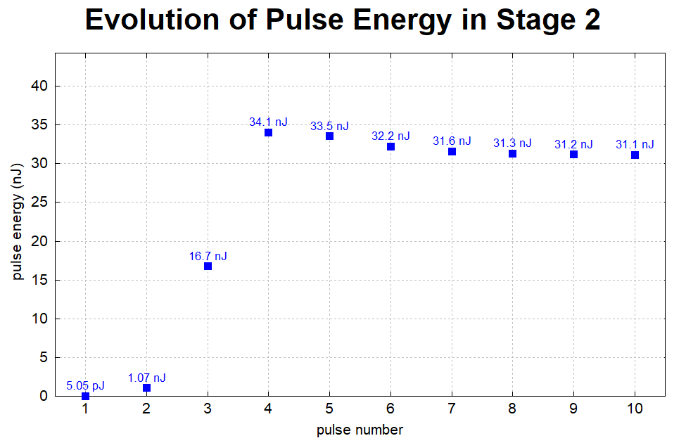
We then simulate ten cycles of pumping and pulse amplification with a repetition rate of 5 kHz. Here you see the evolution of pulse energies coming from the first stage:

evolution of pulse energies after stage 1

The same for the second stage:

evolution of pulse energies after stage 2

Another diagram also helps us to inspect other things, such as the build-up of Yb excitation over the pumping cycles:

You see that after ten cycles, the system has essentially reached the steady state. It may be surprising that the output pulse energy of the second stage drops somewhat after the fourth pulse, although the output energy of the first stage is still rising a bit, as is the Yb excitation in the second stage. However, the pulse spectrum broadens and extends far into the longer-wavelength region where the gain is substantially lower. You can see that in the next screenshot.

There are nice diagrams for the output pulses, but you can also use the interactive pulse display window to conveniently inspect the pulses at different locations inside the fiber:

interactive pulse display window

This shows that the pulses are severely distorted after the second amplifier stage; the high peak power leads to strong nonlinear effects, and chromatic dispersion also plays an important role.

This is just one example for possibly unexpected behavior which you can find and analyze with such a simulation model.

In practice, one would probably like to further optimize this amplifier design before implementing it — saving plenty of resources compared with a trial-and-error approach in the lab, which would be expensive and time-consuming.

The simulation form offers convenient additional features, such as efficiently simulating some pre-cycles (automatically stopping when the steady state is reached) before what is shown in the diagram. Also, you could have the initial state of the amplifier based on the signal average input power, which is often close to the steady state.

Case Studies

The following case studies are available, where we used this Power Form:

Case Studies

Soliton Pulses in a Fiber Amplifier

We investigate to which extent soliton pulses could be amplified in a fiber amplifier, preserving the soliton shape and compressing the pulses temporally.

#amplifiers#pulses#nonlinearities

Case Studies

Raman Scattering in a Fiber Amplifier

We investigate the effects of stimulated Raman scattering in an ytterbium-doped fiber amplifier for ultrashort pulses, considering three very different input pulse duration regimes. Surprisingly, the effect of Raman scattering always gets substantial only on the last meter, although the input peak powers vary by two orders of magnitude.

#amplifiers#pulses#nonlinearities