GitHub - ponnhide/patchworklib: Patchwork for matplotlib: A subplot manager for intuitive layouts in matplotlib, seaborn, and plotnine. (original) (raw)
patchworklib
Patchworklib is a universal composer of matplotlib-related plots (simple matplotlib plots, Seaborn plots (both axis-level and figure-level), and plotnine plots). This library is inspired by patchwork for ggplot2. Accordingly, as original patchwork, users can easily align matplotlib plots with only "/" and "|" operators. Although a good subplot composer, "subplot_mosaic" is provided from matplotlib formally, I believe the way of patchworklib is more straightforward and more flexible.
Additionally, several third-party libraries based on matplotlib, such as plotnine and seaborn, provide functions to generate beautiful plots with simple python codes, but many of those plots cannot be handled as matplotlib subplots. Therefore, their placement must be adjusted manually. Now, scientists spend their valuable time arranging figures.
Patchworklib provides a solution for the problem. By using patchworklib, any kind of seaborn and plotnine plots can be handled as matplotlib subplots.
Join Our Team: Bioinformatics Researcher Wanted.
We are currently seeking a skilled researcher with expertise in bioinformatics to join our lab.
For more details and to apply, please visit the following URL.
Installation
For normal users, we recommended you to install the official release as follows.pip install patchworklib
If you want to use developmental version, it can be installed using the following single command:pip install git+https://github.com/ponnhide/patchworklib.git
News
10122024: version 0.6.5 is released.
- Seaborn v0.13.X is now supported.
- plotnine v0.13.6 might be supported.
10232023: version 0.6.3 is released.
- Seaborn v0.13.0 is now supported.
- I have confirmed patchworklib still works for plotnine v0.12.3.
05162023: version 0.6.1 was released.
- I could not fully support plotnine version 0.12.1 (It works, but patchworklib arrangement results are not as expected). Maybe, I will do not support plotnine in the future.
- Bricks object gained the new methods
align_xlabelsandalign_ylabels, which help users align x/y labels of the given Brick object. - The new argument
equal_spacingwas added to the stack function. If this value isTrue, axes bounding-boxes should be placed with equal spacing between them. Otherwise, depending on the text values of x/y tick labels and x/y labels, they may not always be equally spaced. - Closed and maybe solved the issue "Align labels of Bricks when subplot axes are aligned. #40"
- Closed and maybe solved the issue "Doesn't work with Plotnine Seaborn Theme. #37"
- Closed and maybe solved the issue "The position of the title cannot be set in plotnine. #36"
Change log
#### 12082022: version 0.5.0 was released. - New operators, "+" and "-", were added. - plotnine > v0.10.x is now supported. - Plots generated by object-oriented seaborn interface can now be handled by patchworklib. - Descriptions of each function and class provided in patchworklib was added to this repository. If you want to know how to use patchworklib in detail, please see [API.md](https://github.com/ponnhide/patchworklib/blob/main/API.md). - Updated [patchworklib-examples](https://github.com/ponnhide/patchworklib-examples)
08152022: Version 0.4.7 was released.
- A few bugs were fixed.
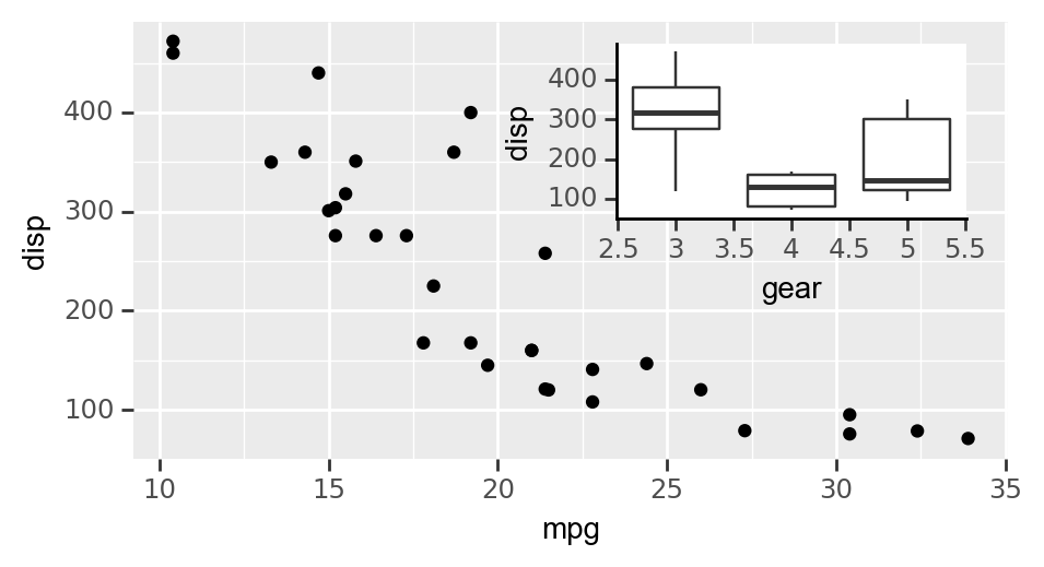
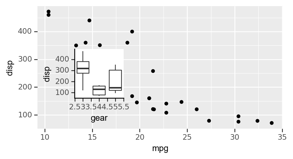
- Add inset function. please see the following example.
- Add
keep_aspectparameter tohstackandvstackfunciton. - Example codes were moved to patchworklib-examples Create an inset element
import patchworklib as pw from plotnine import * from plotnine.data import *
g1 = pw.load_ggplot(ggplot(mtcars) + geom_point(aes("mpg", "disp")),figsize=(4, 2)) g2 = pw.load_ggplot(ggplot(mtcars) + geom_boxplot(aes("gear", "disp", group = "gear")) + theme_classic()) g12 = pw.inset(g1,g2) g12.savefig()
g12 = pw.inset(g1,g2, loc="lower left", hratio=0.4, wratio=0.2) g12.savefig("inset_plotnine2.png")
08092022: Version 0.4.6 was released.
- A few bugs were fixed (See issue #18).
- Plotting speed was improved.
07202022: Version 0.4.5 was released.
- A few bugs were fixed.
- Modified functions relating to the inheritance of the ggplot theme. If you use patchworklib for handling plotnine plots, please do update.
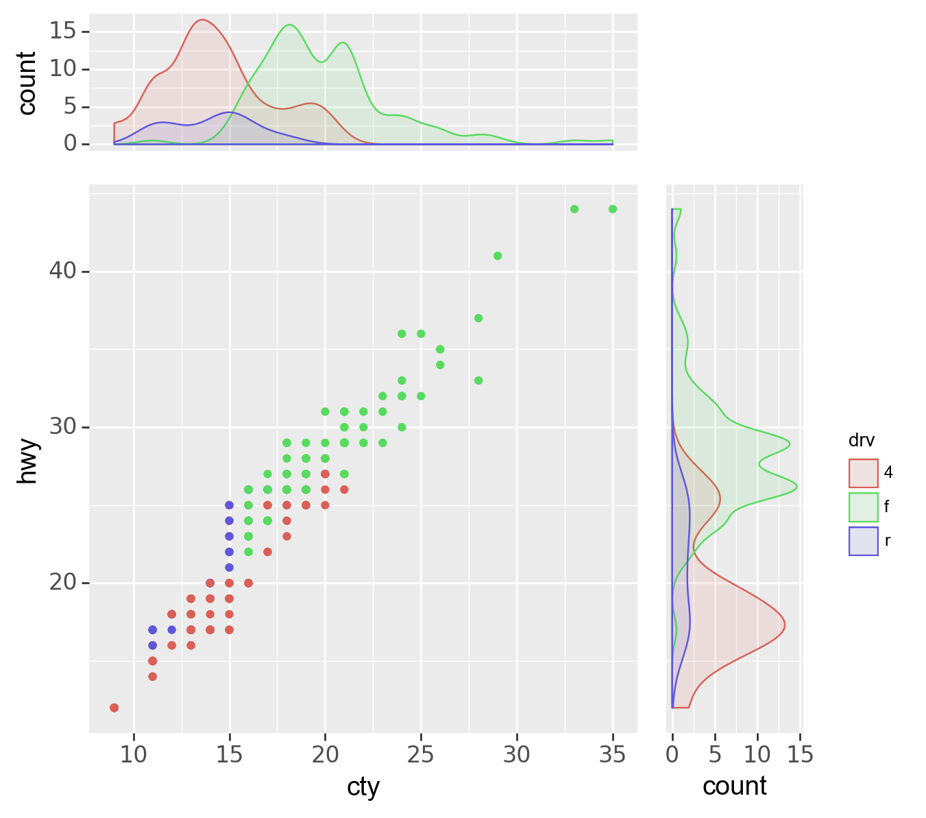
- When specifying a plot (Brick object) in Bricks object, you can specify the Brick object directly instead of the label name of the Brick object. Please see the following example. Alignment of a plotine plot by specifying a Brick object in the Bricks object.
import patchworklib as pw from plotnine import * from plotnine.data import *
g1 = pw.load_ggplot(ggplot(mpg, aes(x='cty', color='drv', fill='drv')) + geom_density(aes(y=after_stat('count')), alpha=0.1) + scale_color_discrete(guide=False) + theme(axis_ticks_major_x=element_blank(), axis_text_x =element_blank(), axis_title_x=element_blank(), axis_text_y =element_text(size=12), axis_title_y=element_text(size=14), legend_position="none"), figsize=(4,1))
g2 = pw.load_ggplot(ggplot(mpg, aes(x='hwy', color='drv', fill='drv')) + geom_density(aes(y=after_stat('count')), alpha=0.1) + coord_flip() + theme(axis_ticks_major_y=element_blank(), axis_text_y =element_blank(), axis_title_y=element_blank(), axis_text_x =element_text(size=12), axis_title_x=element_text(size=14) ), figsize=(1,4))
g3 = pw.load_ggplot(ggplot(mpg) + geom_point(aes(x="cty", y="hwy", color="drv")) + scale_color_discrete(guide=False) + theme(axis_text =element_text(size=12), axis_title=element_text(size=14) ), figsize=(4,4))
pw.param["margin"] = 0.2 (g1/(g3|g2)[g3]).savefig() #By specifying g3 in (g3|g2), g1 is positioned exactly on g3.
07192022: Version 0.4.3 was released.
- A few bugs were fixed.
basefigureparameter was added. You can access the base figure of patchworklib bypatchworklib.basefigure- plotnine v0.9.0 was now supported. Probably, it still have some bugs. If you find bugs, please let me know on the issue.
04222022: Version 0.4.2 was released.
- A few bugs were fixed.
04182022: Version 0.4.1 was released.
load_seaborngridcan accepts aseaborn.clustermapplot. For details, see example code on Google colab- A few bugs were fixed.
03272022: Version 0.4.0 was released.
- Add docstring for each method and class.
- Add several new methods of
patchworklib.Bricksclass to set common label, title, spine and colorbar forBrickobjets in theBricksobject.
For usage, please refer to the docstring or the example codes on Google colab.
02042022: Version 0.3.6 was released.
- A few bugs relating with the function to arrange multiple polar plot objects.
02042022: Version 0.3.5 was released.
- A few bugs in
move_legendwere fixed. (Themove_legendfor seaborn grided plot was not working properly.) - Improved the speed of
savefigoperation.
01242022: Version 0.3.3 was released.
- A few bugs were fixed.
01222022: Version 0.3.0 was released.
Patchworklib now supports the function to arrange matplotlib.projections.polar.PolarAxes ojbects.
When you load a matplotlib.projections.polar.PolarAxes object as a Brick class object, please use 'cBrick' instead of 'Brick'. Now, you can arrange multiple circos plots using pycircos and patchworklib. Please see the following example code.
https://colab.research.google.com/drive/1tkn7pxRqh9By5rTFqRbVNDVws-o-ySz9?usp=sharing
01212022: Version 0.2.1 was released.
- A few bugs for 'load_seaborngrid' were fixed.
01202022: Version 0.2.0 was released.
Patchworklib is now possible to arrange Seabron gridded plots. The "stack" function is added. A few bugs were fixed.
Arranging seaborn gridded plots
Patchworklib supported the function to arange multiple seborn plots generated based on axisgrid (FacetGrid, PairGrid, and JointGrid). Let's see the follwoing example.
import os import seaborn as sns import patchworklib as pw from functools import reduce pw.overwrite_axisgrid() #When you use pw.load_seagorngrid, 'overwrite_axisgrid' should be executed.
df = sns.load_dataset("penguins") g1 = sns.pairplot(df, hue="species") g1 = pw.load_seaborngrid(g1) g1.move_legend("upper left", bbox_to_anchor=(0.08,1.01))
planets = sns.load_dataset("planets") cmap = sns.cubehelix_palette(rot=-.2, as_cmap=True) g2 = sns.relplot( data=planets, x="distance", y="orbital_period", hue="year", size="mass", palette=cmap, sizes=(10, 200), ) g2.set(xscale="log", yscale="log") g2.ax.xaxis.grid(True, "minor", linewidth=.25) g2.ax.yaxis.grid(True, "minor", linewidth=.25) g2.despine(left=True, bottom=True) g2 = pw.load_seaborngrid(g2)
penguins = sns.load_dataset("penguins") g3 = sns.jointplot( data=penguins, x="bill_length_mm", y="bill_depth_mm", hue="species", kind="kde", ) g3 = pw.load_seaborngrid(g3, labels=["joint","marg_x","marg_y"]) ((g2/g3["marg_x"])|g1).savefig()
Also, some example codes are made executable in Google Colaboratory.
"stack" fucntion
I implemented the stack function. This function allows users to arrange multiple (more than two) Brick or Bricks objects along the specified direction as follows.
import patchworklib as pw ax_list = [] for i in range(10): ax_list.append(pw.Brick(figsize=(2,2), label="ax{}".format(i))) stacked_axes = pw.stack(ax_list, operator="|", margin=0.2) stacked_axes.savefig()
01142022: Version 0.1.0 was released.
- Patchworklib was now avialable through pip. 01132022: "spacer" class was implemented and "case" parameter was added to Bricks class.
Add empty spaces around a plot
#preparation of plot data import numpy as np import matplotlib as mpl import patchworklib as pw
data1 = 20 * np.random.rand(100,100) - 10 data2 = 20 * np.random.rand(100,100) - 10 cmap = mpl.cm.Reds norm = mpl.colors.Normalize(vmin=-10, vmax=10) ax1 = pw.Brick("axx", figsize=(3,3)) ax2 = pw.Brick("axy", figsize=(3,3)) ax1.imshow(data1, interpolation='nearest', cmap=cmap, aspect="auto") ax2.imshow(data2, interpolation='nearest', cmap=cmap, aspect="auto")
w/o spacer
ax_cb = pw.Brick("ax_cb", figsize=(0.1,3)) cb = mpl.colorbar.ColorbarBase(ax_cb, cmap=cmap, norm=norm) ax12 = ax1|ax2 heatmap2 = ax12 | ax_cb heatmap2.savefig()
w/ spacer
ax_cb2 = pw.Brick("ax_cb2", figsize=(0.1,1.5)) cb2 = mpl.colorbar.ColorbarBase(ax_cb2, cmap=cmap, norm=norm) heatmap2 = ax12 | (pw.spacer(ax_cb2,0.5)/ax_cb2/pw.spacer(ax_cb2,0.5)) heatmap2.savefig()
Super titile for multiple plots
Sometimes, all that is needed to have common labels and title for multiple plots.
By specifying case parameter of a Bricks class object, common matplotlib artist ojbects for multiple plots can be handled.
ax12.case.set_title("A global title for multiple plots", pad=10) heatmap2 = ax12|(pw.spacer(ax_cb,0.5)/ax_cb/pw.spacer(ax_cb,0.5)) heatmap2.savefig("")
 01072022: Patchworklib was updated to allow arranging multiple plots generated by plotnine.
import patchworklib as pw from plotnine import * from plotnine.data import * g1 = pw.load_ggplot(ggplot(mtcars) + geom_point(aes("mpg", "disp")) + theme(figure_size=(2, 3))) g2 = pw.load_ggplot(ggplot(mtcars) + geom_boxplot(aes("gear", "disp", group = "gear")) + theme(figure_size=(2, 3))) g12 = g1 | g2 g12.savefig()
g3 = pw.load_ggplot(ggplot(mpg, aes(x='displ', y='hwy')) + geom_point() + geom_smooth(span=.3) + theme(figure_size=(2, 3))) g4 = pw.load_ggplot(ggplot(mtcars) + geom_bar(aes("carb")) + theme(figure_size=(7, 2))) g1234 = (g1|g2|g3)/g4 g1234.savefig()
Usage
If you want to know how to use patchworklib in detail, please see API.md.
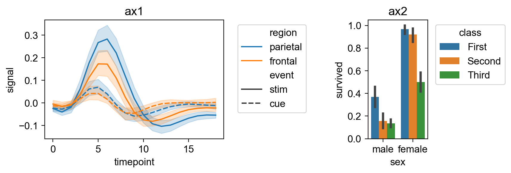
Using patchworklib, you can quickly and freely arrange matplotlib plots with only | and / oparators as follows.
import patchworklib as pw import seaborn as sns
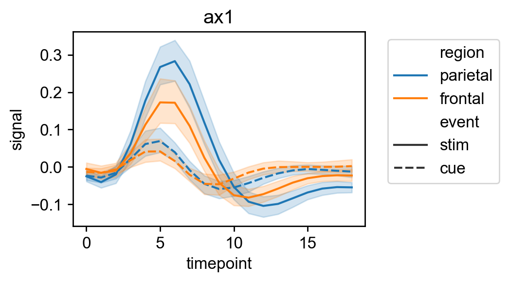
fmri = sns.load_dataset("fmri") ax1 = pw.Brick(figsize=(3,2)) sns.lineplot(x="timepoint", y="signal", hue="region", style="event", data=fmri, ax=ax1) ax1.legend(bbox_to_anchor=(1.05, 1.0), loc='upper left') ax1.set_title("ax1")
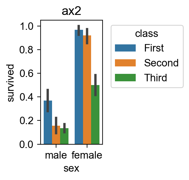
titanic = sns.load_dataset("titanic") ax2 = pw.Brick(figsize=(1,2)) sns.barplot(x="sex", y="survived", hue="class", data=titanic, ax=ax2) ax2.move_legend(new_loc='upper left', bbox_to_anchor=(1.05, 1.0)) ax2.set_title("ax2")
ax12 = ax1|ax2 ax12.savefig("ax12.png")
Jupyter Notebook files for all of the example codes are provided in patchworklib-examples and also made executable in Google Colaboratory.
- tutorial: Basic example codes of patchworklib
- subplots for plotnine: Arranging plotnine plots using patchworklib
- subplots for seaborngrid: Arranging figure-level seaborn plots using patchworklib
- placing_super_elements: Placing super labels and spines for a set of multiple subplots.
Also, please see https://python.plainenglish.io/a-subplot-manager-for-intuitive-layout-in-matplotlib-bd037fe967f4
Gallery
Arrangement of multiple axis-level seaborn plots 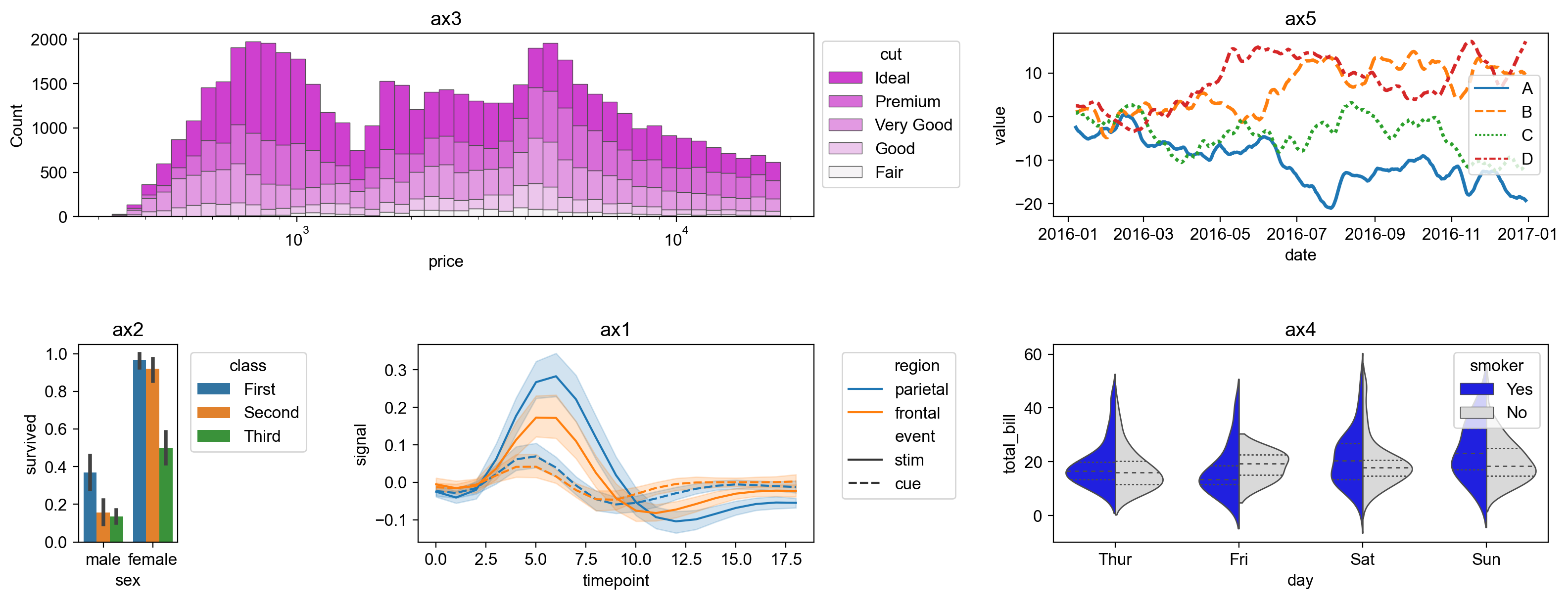
Arrangement of multiple Plotnine plots 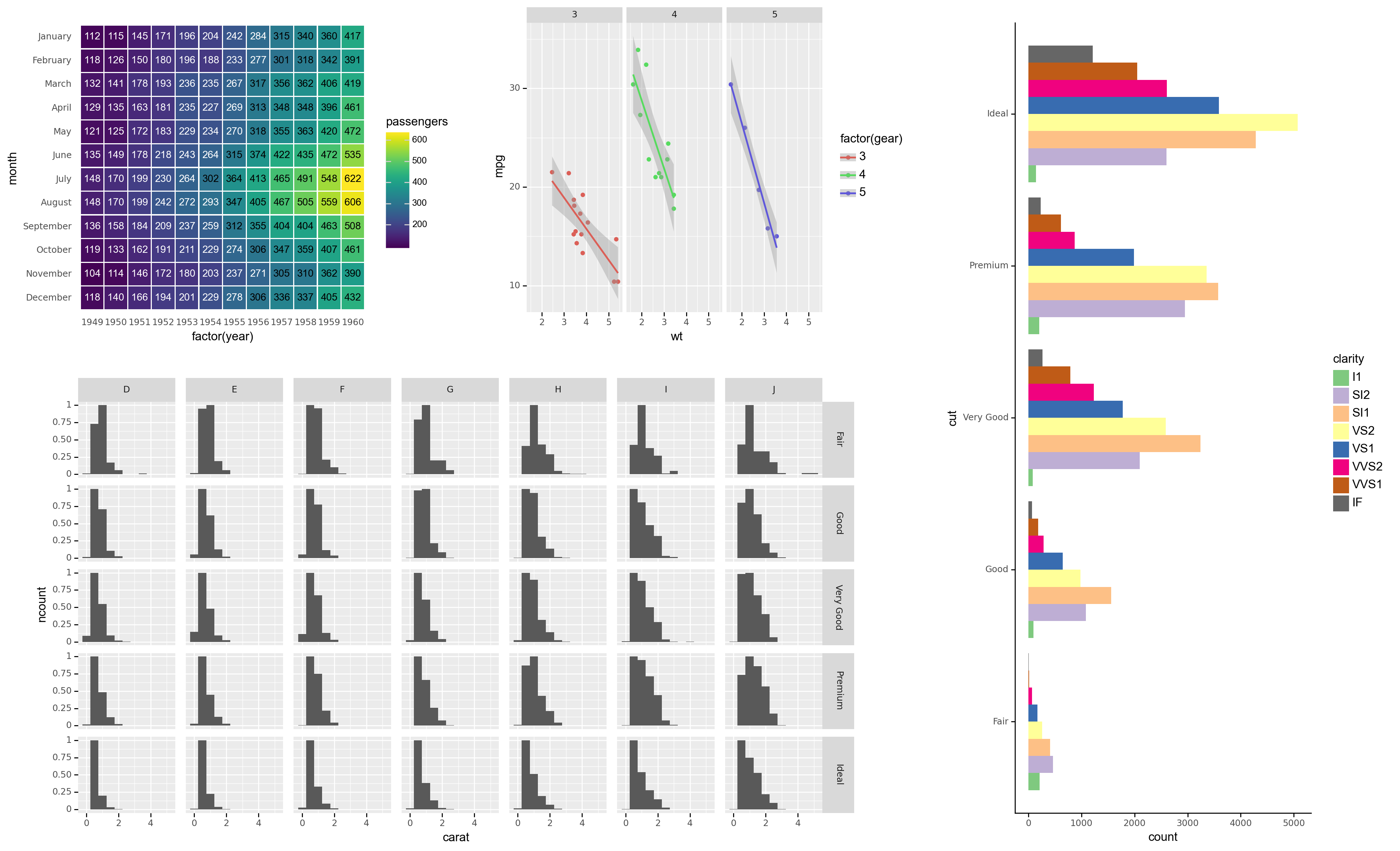
Arrangement of multiple figure-level seaborn plots 
Getting started
Example codes
Tutorial ~_Compose multiple seaborn plots_~The follwoing tutorial codes can be executable in tutorial1
1. Importing patchworklib library
import patchworklib as pw fmri = sns.load_dataset("fmri") ax1 = pw.Brick("ax1", figsize=(4,2)) sns.lineplot(x="timepoint", y="signal", hue="region", style="event", data=fmri, ax=ax1) ax1.move_legend(new_loc='upper right') ax1.set_title("ax1")
2. Creating example plots
Creating some example plots using the searborn module. Brick class provided by the patchworklib module is implemented as subclass of matplotlib.axes.Axes. Therefore, Brick class object can be given to the seaborn plot functions that have the ax parameters.
When creating a Brick class object, the label value should be specified, and it should be unique among the Brick class objects generated in the python script (If the label value is not specified, the unique label name is automatically given. By using get_label() method, the value can be confirmed). The figisize parameter can also be specified. However, the value is not very important because the figure size of Brick class objects can be automatically adjusted in arranging the plots. The savefig( filename=str) method returns matplotlib.figure.Figure class object. If filename is given, the figure object can be output to the file.
import seaborn as sns #Example plot 1 (ref: https://seaborn.pydata.org/examples/errorband_lineplots.html) fmri = sns.load_dataset("fmri") ax1 = pw.Brick("ax1", figsize=(4,2)) sns.lineplot(x="timepoint", y="signal", hue="region", style="event", data=fmri, ax=ax1) ax1.move_legend(new_loc='upper right') ax1.set_title("ax1") ax1.savefig()
Brick class provides the movelegend( loc=str, bboxtoanchor=(float,float)) method. By using this method, legend location can be quickly modified.
#Example plot 2 (ref: https://seaborn.pydata.org/tutorial/categorical.html) titanic = sns.load_dataset("titanic") ax2 = pw.Brick("ax2", figsize=(1,2)) sns.barplot(x="sex", y="survived", hue="class", data=titanic, ax=ax2) ax2.move_legend(new_loc='upper left', bbox_to_anchor=(1.05, 1.0)) #Original method of Blick class ax2.set_title("ax2") ax2.savefig()
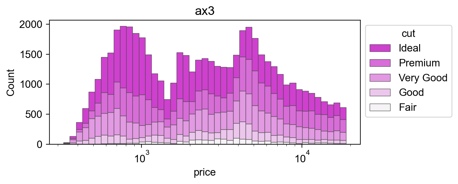
#Example plot 3 (ref: https://seaborn.pydata.org/examples/histogram_stacked.html) diamonds = sns.load_dataset("diamonds") ax3 = pw.Brick("ax3", (5,2)) sns.histplot(diamonds, x="price", hue="cut", multiple="stack", palette="light:m_r", edgecolor=".3", linewidth=.5, log_scale=True, ax = ax3) ax3.set_title("ax3") ax3.savefig()
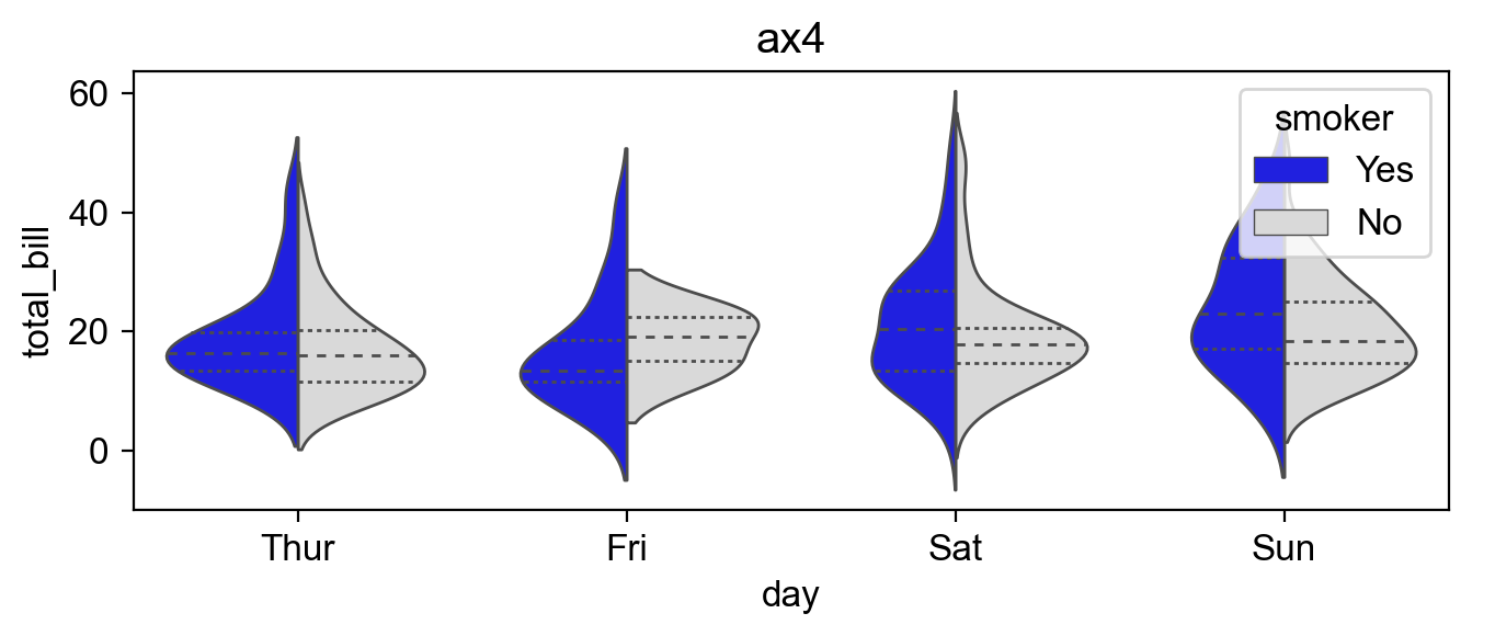
#Example plot 4 (ref:https://seaborn.pydata.org/examples/grouped_violinplots.html) tips = sns.load_dataset("tips") ax4 = pw.Brick("ax4", (6,2)) sns.violinplot(data=tips, x="day", y="total_bill", hue="smoker", split=True, inner="quart", linewidth=1, palette={"Yes": "b", "No": ".85"}, ax=ax4) ax4.set_title("ax4") ax4.savefig("../img/ax4.png")
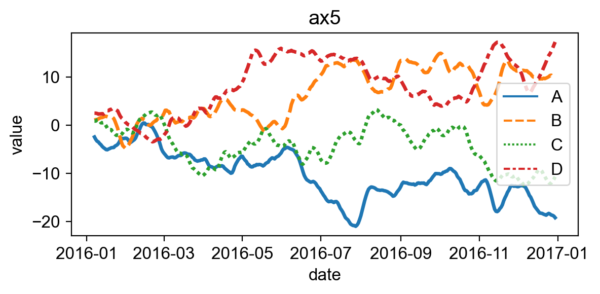
#Example plot 5 (ref:https://seaborn.pydata.org/examples/wide_data_lineplot.html) rs = np.random.RandomState(365) values = rs.randn(365, 4).cumsum(axis=0) dates = pd.date_range("1 1 2016", periods=365, freq="D") data = pd.DataFrame(values, dates, columns=["A", "B", "C", "D"]) data = data.rolling(7).mean() ax5 = pw.Brick("ax5", (5,2)) sns.lineplot(data=data, palette="tab10", linewidth=2.5, ax=ax5) ax5.set_xlabel("date") ax5.set_ylabel("value") ax5.set_title("ax5") ax5.savefig()
3. Arranging and stacking plots
The patchworklib module provides two operators " |", "/" that enable designing tidy layout for multiple plots with simple operations. The "|" operator will place the plots beside each other, while the "/" operator will stack them.
#Arrange "ax1," "ax2," and "ax4" horizontally. ax124 = ax1|ax2|ax4 ax124.savefig("../img/ax124.png")
The object generated by arranging multiple Brick object (Bricks class object) can also be arranged and stacked with other Brick objects. Additionally, It is possible to create more complex layouts by nesting the operations.
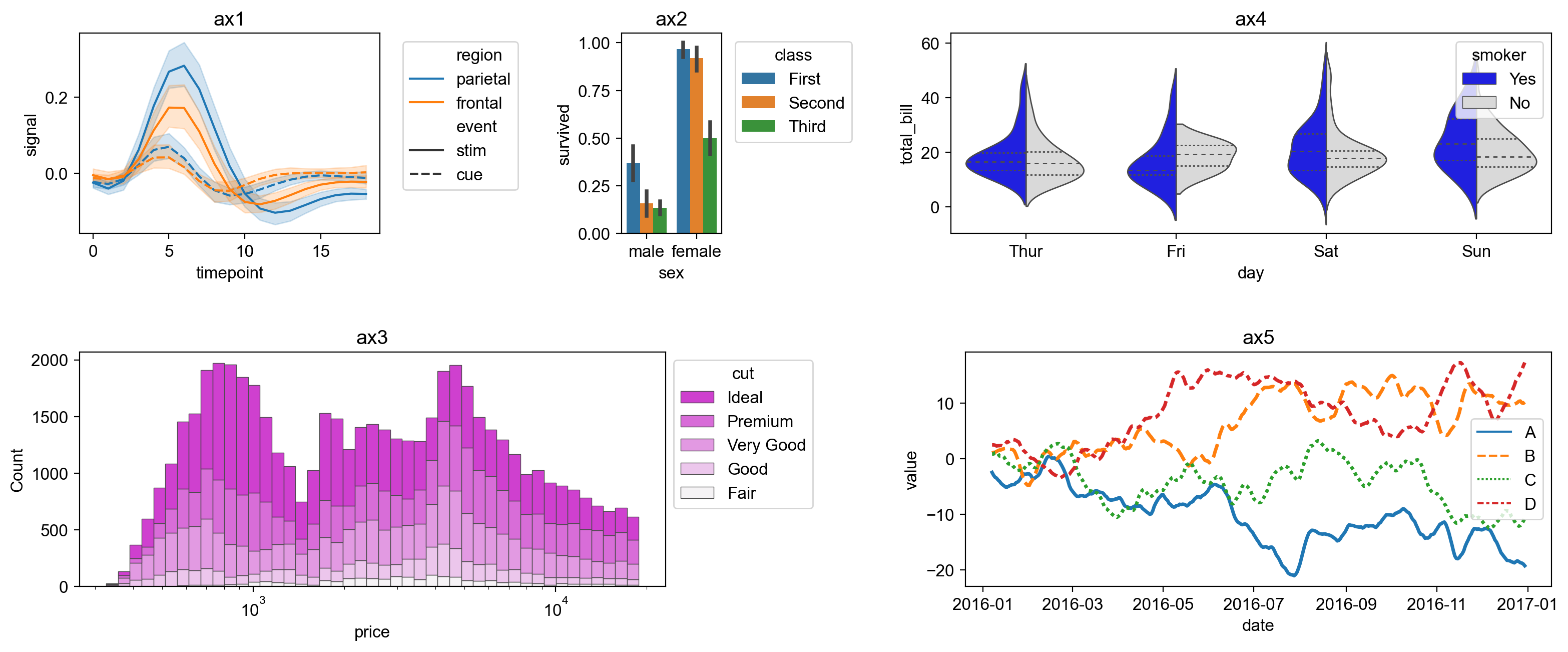
ax12435 = ax124/(ax3|ax5) ax12435.savefig("../img/ax12435.png")
You can quickly test another layout by rearranging them.
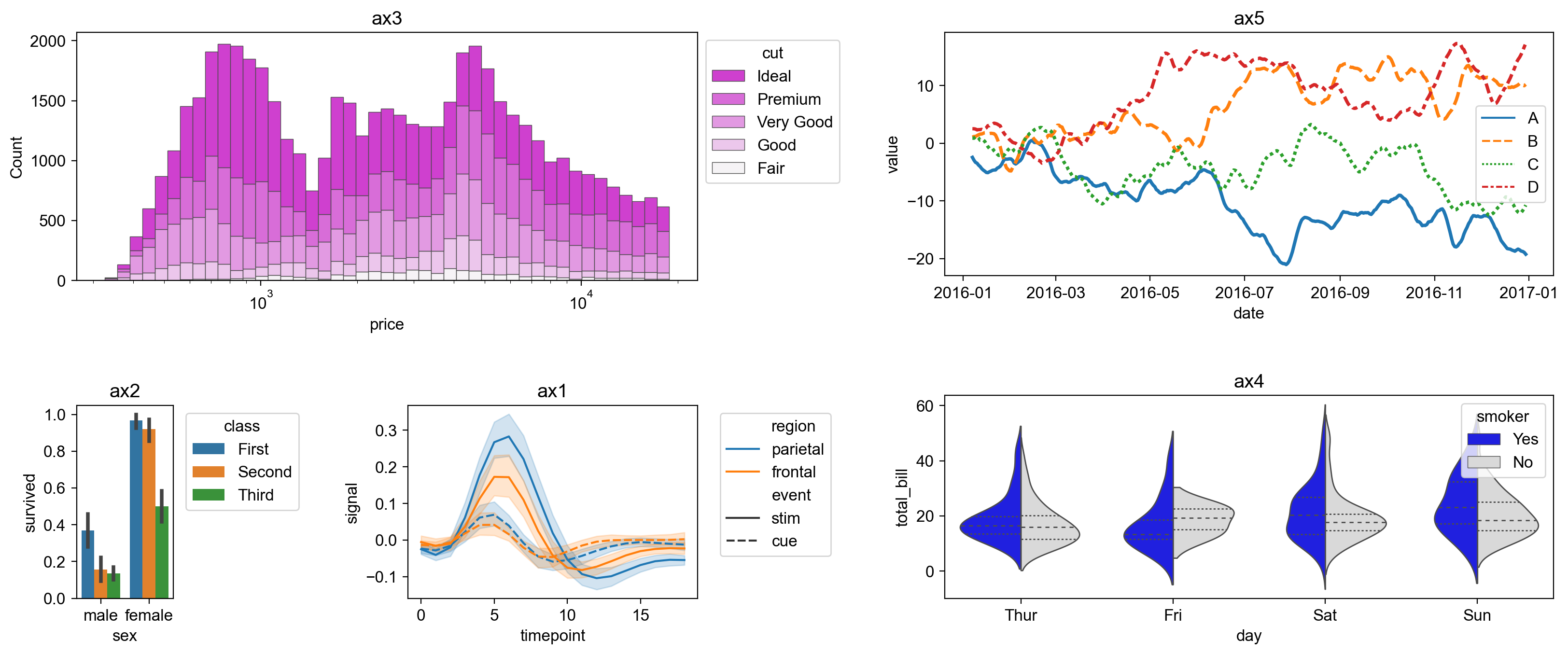
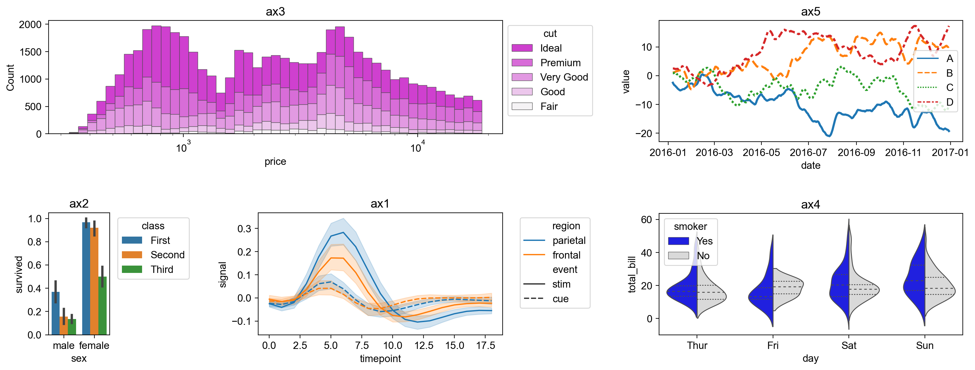
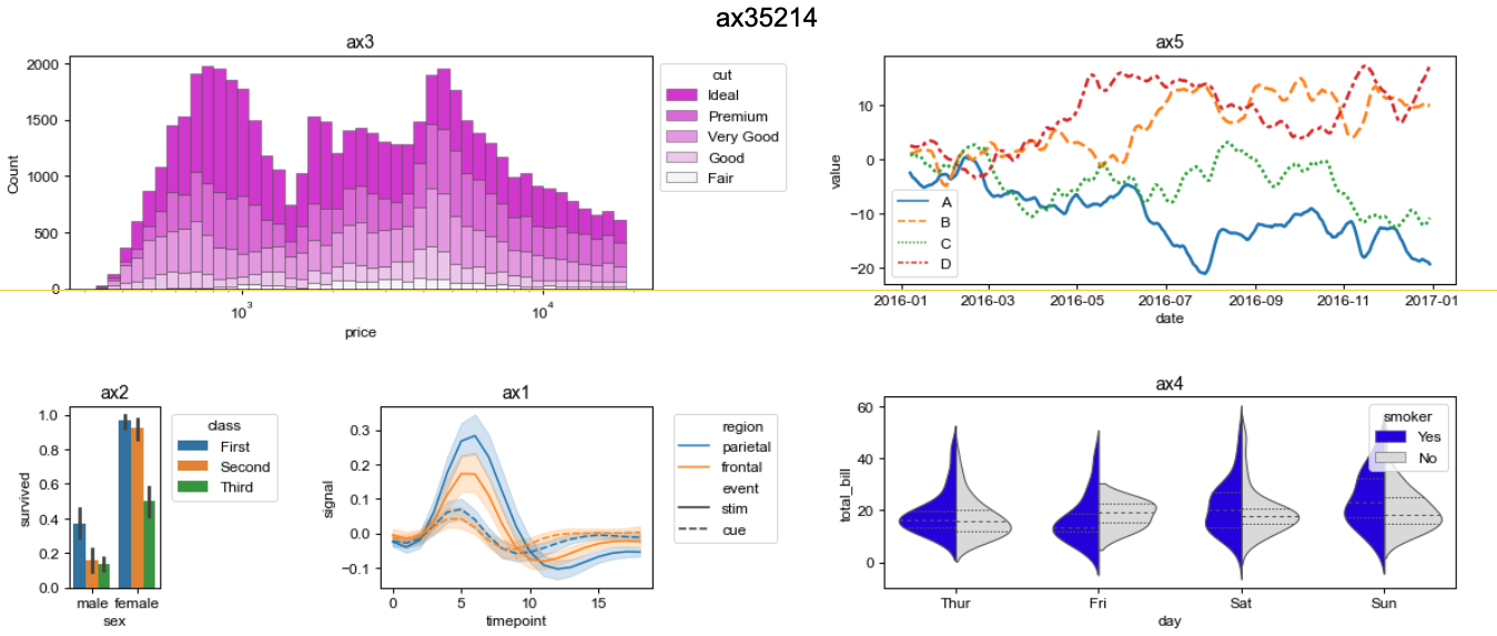
ax35214 = (ax3/(ax2|ax1))|(ax5/ax4) ax35214.savefig()
If you want to adjust the margins between objects, please change the value of .param["margin"].
pw.param["margin"]=0.2 #Default value is 0.5. ax35214 = (ax3/(ax2|ax1))|(ax5/ax4) ax35214.savefig("../img/ax35214_v1.1.png")
Also, the aspect ratios of each plot can be freely modifiable.
pw.param["margin"]=0.5 ax1.change_aspectratio((4,2)) ax3.change_aspectratio((4,1)) ax4.change_aspectratio((5,2)) ax35214_v2 = (ax3/(ax2|ax1))|(ax5/ax4) ax35214_v2.savefig()
4. Packing plots with label indexing (Advanced method)
By specifying the Brick objects in a Bricks object with their label name, you can adjust the position of another Brick object to be packed.
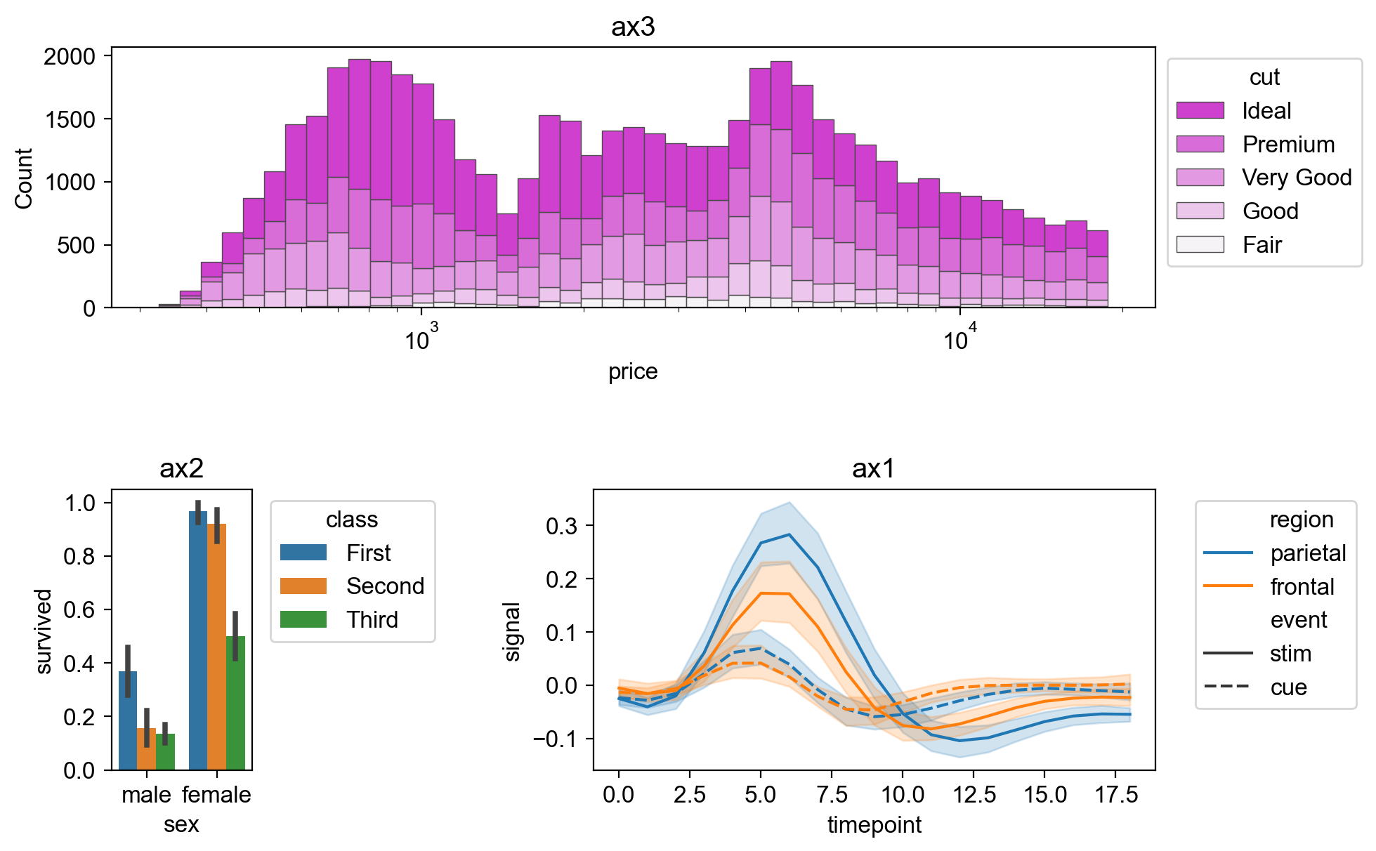
ax321 = ax3/(ax2|ax1) ax321.savefig("../img/ax321.png")
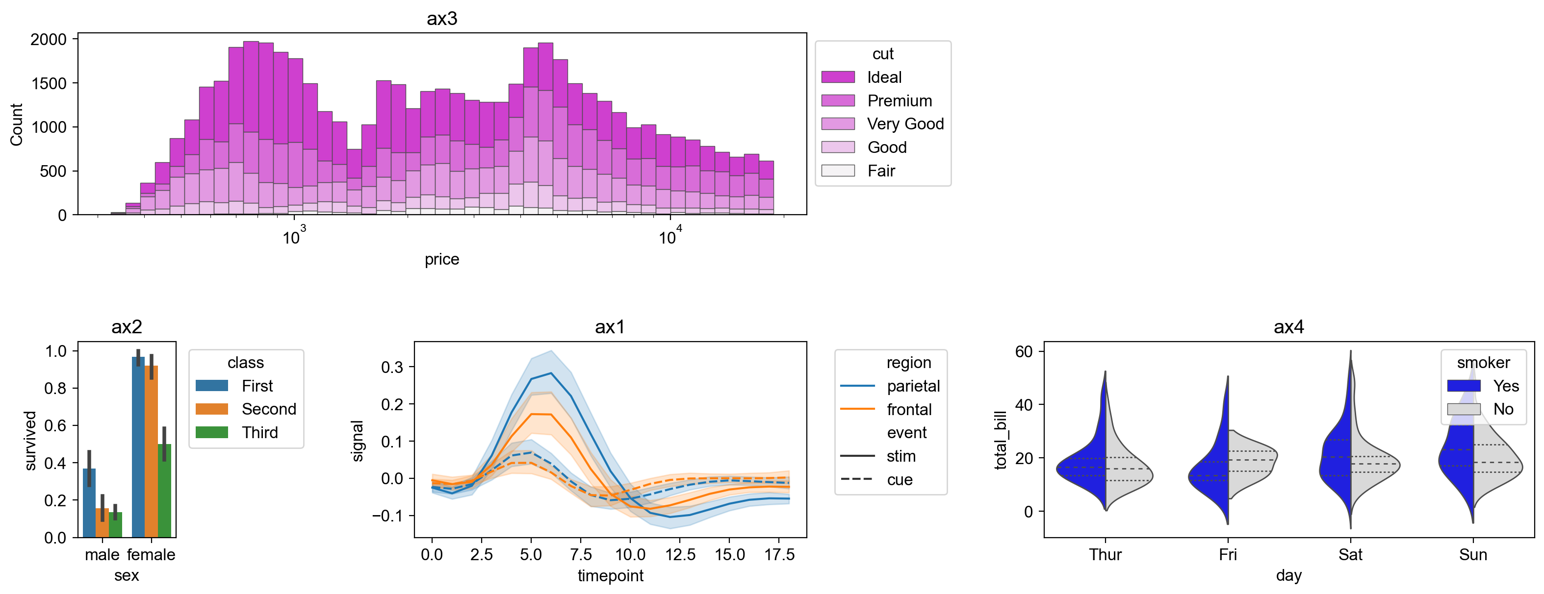
ax3214 = ax321["ax1"]|ax4 ax3214.savefig("../img/ax3214.png")
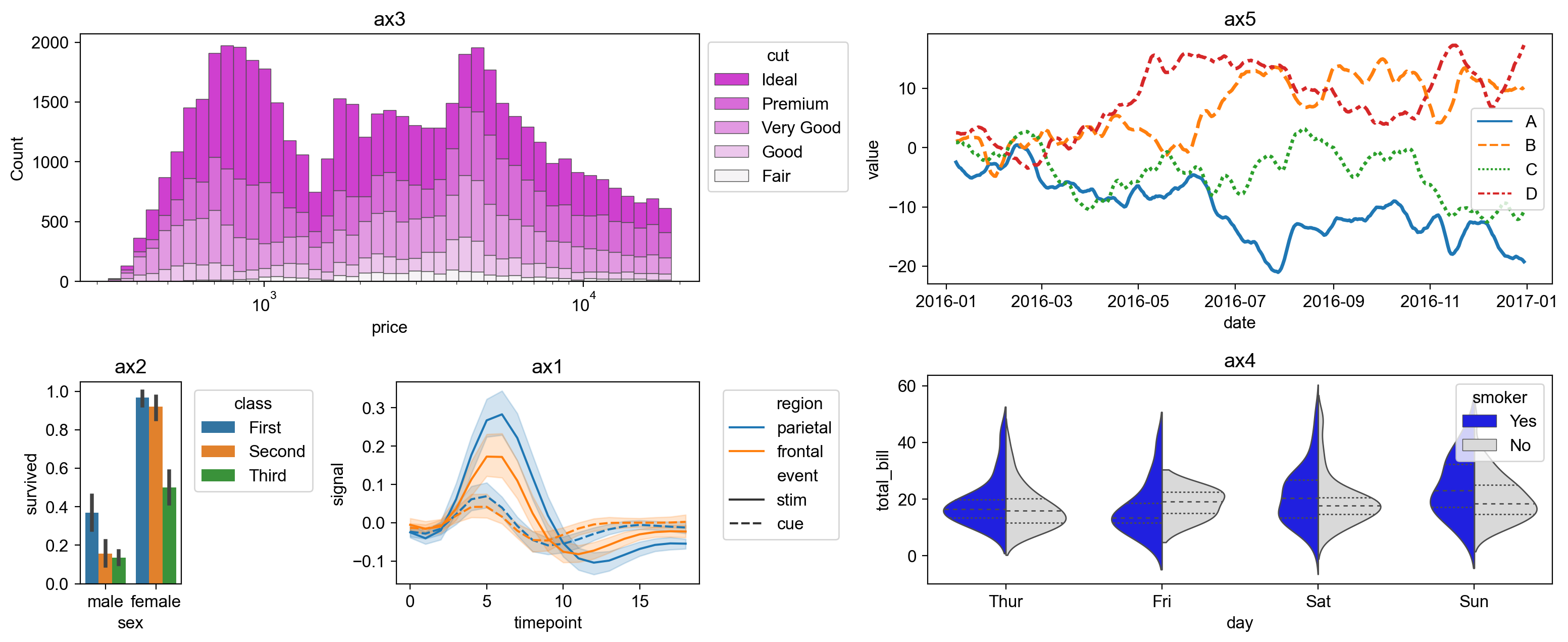
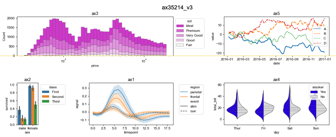
ax35214_v3 = ax3214["ax3"]|ax5 ax35214_v3.savefig("../img/ax35214_v3.png")
The above packing process allows the axes of the objects to be accurately aligned with each other. Actually, in "ax35214" and "ax35214_v2", the bottom axis lines of ax3 and ax5 are not precisely aligned, while in "ax35214_v3", their bottom axis lines are exactly aligned. However, please note that this packing method using label indexing changes aspect ratios of the Brick objects to be packed from the original one to align their axis lines with others.
