A new non-linear normalization method for reducing variability in DNA microarray experiments (original) (raw)
Short abstract
A simple and robust non-linear method is presented for normalization using array signal distribution analysis and cubic splines. Both the regression and spline-based methods described performed better than existing linear methods when assessed on the variability of replicate arrays
Abstract
Background
Microarray data are subject to multiple sources of variation, of which biological sources are of interest whereas most others are only confounding. Recent work has identified systematic sources of variation that are intensity-dependent and non-linear in nature. Systematic sources of variation are not limited to the differing properties of the cyanine dyes Cy5 and Cy3 as observed in cDNA arrays, but are the general case for both oligonucleotide microarray (Affymetrix GeneChips) and cDNA microarray data. Current normalization techniques are most often linear and therefore not capable of fully correcting for these effects.
Results
We present here a simple and robust non-linear method for normalization using array signal distribution analysis and cubic splines. These methods compared favorably to normalization using robust local-linear regression (lowess). The application of these methods to oligonucleotide arrays reduced the relative error between replicates by 5-10% compared with a standard global normalization method. Application to cDNA arrays showed improvements over the standard method and over Cy3-Cy5 normalization based on dye-swap replication. In addition, a set of known differentially regulated genes was ranked higher by the _t_-test. In either cDNA or Affymetrix technology, signal-dependent bias was more than ten times greater than the observed print-tip or spatial effects.
Conclusions
Intensity-dependent normalization is important for both high-density oligonucleotide array and cDNA array data. Both the regression and spline-based methods described here performed better than existing linear methods when assessed on the variability of replicate arrays. Dye-swap normalization was less effective at Cy3-Cy5 normalization than either regression or spline-based methods alone.
Background
Microarray data is almost always described as containing large measurement noise or high variability. Some sources of variability are random but most are systematic and due to specific features of the particular microarray technology. Systematic effects resulting from the biological process under study are of interest whereas other systematic sources should be removed. Normalization methods are required for controlling uninteresting variability and it is our belief that much of the systematic variability in oligonucleotide array data is controllable through careful normalization. Improper normalization can lead to incorrect conclusions or unacceptably high false-positive or false-negative rates. Here we describe qspline, a non-linear method for controlling signal-dependent sources of variability in Affymetrix oligonucleotide array data, and show that the approach can also be applied to cDNA array data.
Few microarray studies quantify specific sources of variability and fewer still suggest methods for controlling them. Much of the literature addressing microarray normalization concerns cDNA array data, whereas only a few examples can be found for oligonucleotide arrays [1,2,3,4]. Here we review microarray normalization techniques, present the qspline method and show its application to Affymetrix oligonucleotide arrays of human T-cell cultures and cDNA arrays of Bacillus subtilis and Arabidopsis thaliana (H. Næsted, A. Holm, H.B. Nielsen, C.A. Harris, M.H. Beale, M. Andersen, O. Mattsson and J. Mundy, unpublished observations). The oligonucleotide array study compares human T-cell cultures infected with human immunodeficiency virus (HIV) to uninfected cultures and the B. subtilis arrays investigate mutant strains for the genes glnA and tnrA. The A. thaliana experiment compares wild-type to mutant strain and in this context is used to illustrate the effects of normalization on a dye-swap experiment.
Linear normalization methods
Linear methods are the predominant means of microarray normalization. Scaling, the simplest linear approach, assumes a linear relationship passing through the origin. Forcing array distributions to have the same central tendency (arithmetic mean, geometric mean, median) can be accomplished by a scaling factor and has been the method chosen by Affymetrix and others [5]. Linear regression [6,7] and general linear modeling such as ANOVA [8,9] provide offsets, scaling factors and other parameters, but again assume linear relationships and properties of the data or log data distributions, such as normality, that are not always true. In all cases, linear approaches will fall short when the signal bias is not linear.
Approaches for two-channel cDNA arrays apply scaling in order to zero a central tendency of the log expression ratios [10,11,12]. These approaches may also be applied to pairs of single-channel oligonucleotide arrays. Applying an additive offset to the log data is equivalent to a multiplicative scaling of one channel before taking the log. Moving the median or mode of the log-ratios to zero makes the assumption that the majority of genes are not differentially regulated. Additional steps may scale the log-ratios by a measure of dispersion such as the standard deviation or median absolute deviation (MAD), possibly grouping spots according to the printing-tip. This is equivalent to raising both channels to a power before taking the log and is therefore a non-linear transformation of the original signals though giving rise to a linear transformation of the log-signals. Unfortunately, systematic biases are not always linear in log-space either.
Non-linear normalization methods
Non-linear normalization methods have been shown to control signal-dependent non-linear bias between Cy5 and Cy3 channels of cDNA arrays [11,13]. The promising approach of Yang et al. [11] uses lowess local regression [14] directly to paired data as a function of signal intensity. For the cDNA data used by Yang et al. and Tseng et al. [11,13], lowess was used for local linear regression of log(R)-log(G) versus 1/2(log(R) + log(G)) where R, and G are the intensities of the Cy5 and Cy3 channels respectively. Rather than regressing log(R) directly to log(G), these approaches correctly attribute uncertainty to both channels by regressing to the geometric mean of the intensity. Even so, standard regression techniques can be sensitive to outliers, which are likely to occur in microarray data. Robust regression techniques, as found in the R version of lowess [15], are relatively insensitive to outliers. Robust regression techniques incur significant computational costs and, in practice, a small random sample of data must be used for today's oligonucleotide arrays. The approach taken by Tseng et al. [13] and Schadt et al. [4] addresses the outlier issue by selecting non-regulated features based on a rank invariant criterion where all signals from both arrays are sorted and signals with ranks deviating by less than a threshold are included. Normalization of replicate arrays raises the question of which signals should be excluded when none of the genes are differentially expressed. In the method we will describe, no data need to be excluded for curve fitting and it is therefore global and unbiased by subset selection.
Signal-dependent non-linear normalization
The goal of signal-dependent normalization is to make signal distributions comparable across the intensity range. This suggests that the expectation for the difference of paired measurements, or log-ratios, should not significantly deviate from zero anywhere over the intensity range. Again, this is the motivation for centering Cy5 to Cy3 log-ratio distributions of cDNA arrays, but now we consider multiple arrays. If the log-ratio distributions between arrays or color channels are to be centered across the intensity range, then the resulting correlation will be linear with intercept zero and slope one. The resulting data correlation will retain stochastic noise and, more important, the biological variation. This linear data correlation presupposes that the distributions of signals be roughly the same. Our approach seeks to transform the distribution of one array to the distribution of a target array in order to achieve this goal. If the target array is chosen to be the geometric mean probe intensities over the arrays in an experiment, then each array distribution is fitted to an empirical estimate of the signal distribution for the experiment. In principle, any measure of central tendency may be used, although the geometric mean is a natural extension of existing cDNA methodologies. Alternatively, each array can be fitted to the theoretical quantiles of a known distribution (for example, the log-normal distribution). This approach was not chosen here as the observed distributions did not fit a theoretical model and contained well determined, systematic features. In this work we seek only to make the distributions similar to each other whatever those distributions may be.
For Affymetrix data, all the arrays of an experiment can be used to define a target array and thus a target distribution that all arrays are normalized to. As a result of the dye effects, data from two-channel cDNA arrays display significantly different Cy3 and Cy5 signal distributions, suggesting that means calculated over both signal types may not make sense for the definition of a target distribution. Instead, either the geometric mean of the Cy3 or Cy5 channels are used, and all channels from all arrays are normalized to a single Cy3 or Cy5 distribution. This accomplishes both Cy3 to Cy5 normalization within and between arrays. The approach described here can be used to normalize the Cy3 channel to the Cy5 channel within a single array or may also be applied to pairs of Affymetrix arrays.
Qspline normalization
The normalization method described in this work, qspline, uses quantiles from array signals and target signals, x and v, to fit smoothing B-splines. The splines are then used as signal-dependent normalization functions on the signals of x. The target signals can be from another array or could be means calculated from multiple arrays as just described. Splines are a natural and robust choice in that they are capable of representing almost any smooth relationship and will also work well if data is linearly related. Using quantile information provides a much easier fitting problem and avoids directly fitting the pairwise data which often requires robust regression techniques. An example oligonucleotide array signal distribution and quantile comparison can be seen in Figure 1.
Figure 1.
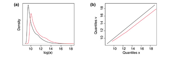
Signal-distribution comparison and QQ correlation plot. (a) Example array distribution plots (left) from kernel smoothed density estimates versus the log intensity data. The target distribution from v (black) is shown alongside that of an example array. (b) The QQ plot shows the correlation of the quantiles from x to the quantiles of the target v and describes a normalizing curve.
Spatial normalization
Spatial heterogeneity of signal can be observed in microarray data and in particular in cDNA microarray data. Variability in Cy3/Cy5 ratios has been shown to be generated, in part, by the specific print-tip used during the spotting of the cDNA probes [11]. In fact, an F-test found that at least one print-tip was very significantly correlated to log-ratio (log(_p_-value) less than -20) in all cDNA arrays used in this study. Spatial effects are not only caused by the printing device but may also be related to; temperature or humidity during the time of printing, the batch of cDNA represented by a specific microtiter plate, reagent flow during the washing procedure after hybridization, or from uneven or tilted glass surfaces during scanning. Microtiter plate effects can appear as vertical or horizontal bands across the array whereas other effects may generate smooth gradients of arbitrary orientation. Signal gradients can be normalized by subtracting local signal estimates (log intensities or log-ratios) and a preliminary approach for this was tested.
These effects, though not as significant as the Cy3 Cy5 bias, can be quite pronounced, as will be observed in the A. thaliana microarrays. Older-generation Affymetrix arrays like those used in this study were subject to local signal biases due to the adjacent placement of probes for each gene-probe set. This bias has since been corrected in more recent oligonucleotide array designs. Other spatial biases can be observed for Affymetrix arrays and are best described as smooth gradients.
Normalization comparison
Log-intensity scaling, lowess and invariant set normalization approaches were compared to qspline for the reduction of variation between replicate arrays in oligonucleotide and cDNA array experiments. Six microarrays were used for each of the HIV and B. subtilis studies. Three control replicate and three treatment replicate single-channel arrays were used in the oligonucleotide array study of HIV-infected T-cells. Six replicate two-channel cDNA arrays provided six control and six treatment channels for each B. subtilis study. In addition, a pair of dye-swapped replicate arrays from A. thaliana were also normalized to investigate the various normalizations methods versus dye-swap normalization.
The lowess normalization method for cDNA array data was taken from the Rarray module of the sma package (version 0.5.8) [16] and was used for the normalization of all cDNA microarray data sets. For oligonucleotide array data, a lowess method was adapted from Raffy module of the sma package. Instead of averaging all pairwise array regressions on a single random sample of feature pairs, iterative regressions between an array and the target array were averaged using a new random sample for each iteration. The former method tended to significantly under-normalize whereas the adapted method used essentially the same procedure but performed significantly better.
In addition to print-tip normalization for cDNA arrays, a spatial gradient normalization was devised using a two-dimensional Gaussian function. This function was used to estimate local background bias over a window of probes for the log-ratios of cDNA and oligonucleotide array data. Log-ratios for oligonucleotide array data were calculated versus the geometric mean of each probe across arrays, as will be seen throughout this work. Lastly, although it is only a matter of preference, we used log base 2 throughout.
Results
Global assessment of normalization
The assessment of normalizations was first observed for global features such as absolute signal distribution and relative signal distribution. Absolute signals result from the image analysis and are the values extracted from the pixel intensities of each spot, whereas relative signals are log-ratios of absolute signals versus measured or calculated background probe signals. The absolute signal distributions of the six oligonucleotide arrays can be seen in Figure 2 for the HIV (perfect-match (PM) distributions) and glnA (Cy3 G and Cy5 R distributions) experiments both before and after normalization. Distributions for replicate arrays or replicated Cy3, Cy5 channels are shown in the same color.
Figure 2.
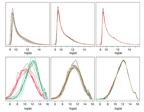
Signal distributions before and after normalization. Density estimates for the six oligonucleotide arrays of the HIV study (top row) and six cDNA arrays of the glnA study (bottom row): before normalization (left column), after lowess normalization (middle column), and after qspline normalization (right column). Scaled print-tip versions of lowess and qspline are shown for the glnA experiment and global lowess and qspline are shown for the HIV experiment. Control samples are shown in green and treatment samples (HIV-infected cells and glnA mutants) in red, along with the geometric means distribution in black for the six HIV arrays and the six Cy3 signals from glnA arrays. Signal distributions were calculated by Gaussian kernel density estimation.
Figure 2 shows that signal-distribution inconsistencies between replicate oligonucleotide arrays are comparable to those between treatments. For this example, distribution discrepancies appear minor though we have encountered Affymetrix experiments showing dramatically disparate distribution profiles. Scaling by the trimmed mean of PM-mismatch (MM), as done by the Affymetrix GeneChip software (MAS 4.0), was observed to separate PM intensity distributions more than is observed for unnormalized data and was not considered in this study. Newer versions of the Affymetrix software (MAS 5.0) incorporate additional log-intensity scaling routines that improve normalization performance but were not investigated in this study. Log-intensity scaling used in this comparison also did not make signal distributions more comparable than the unnormalized case. Both lowess and invariant set normalization methods resulted in similar array distributions, whereas our version of lowess normalization gave more comparable distributions than the Raffy version. The qspline normalization resulted in the most similar array distributions, which are indistinguishable from each other in Figure 2.
Normalized array distributions for the two cDNA experiments showed a similar trend, although cDNA array distributions strongly depended on the cyanine dye and in all cases, distributions were much less smooth. The dye bias can clearly be seen in the unnormalized Cy3 and Cy5 signal distributions shown in green and red respectively in Figure 2. Both global and scaled print-tip lowess and qspline normalizations showed similar signal-distribution comparisons. Lowess and qspline normalizations generated more comparable Cy3 and Cy5 distributions than scaling alone, whereas qspline methods generated the most similar signal distributions.
The effects of normalization on the relative signal distributions, log(xi/v), are shown in Figure 3 for both oligonucleotide and cDNA arrays for the same normalizations shown in Figure 2. These probe-deviation distributions show the variability from each v calculated over all the channels in an experiment and therefore show log-intensity deviations from the experiments' centroid. The original signal intensities are lost in these plots of relative information, but global biases can still be seen. Comparable decreases in global array bias were observed for lowess, qspline and invariant set normalized results. Systematic differences between cDNA Cy3 and Cy5 channel distributions can be seen before normalization but display similar distributions after signal-dependent normalization. By visual inspection, print-tip scaling followed by qspline normalization resulted in the greatest decrease of relative signal bias for the cDNA array data. Little if any difference was observed between global lowess and scaled print-tip lowess with regard to relative signal distributions. The same was observed for the two variants of qspline, suggesting that print-tip effects are much smaller than the global biases. The same trends were observed for the four channels of the dye-swap replicate cDNA arrays.
Figure 3.
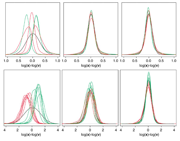
Relative signal distributions before and after normalization. Relative signals (log-ratios) log(x)-log (v), for oligonucleotide arrays (HIV, top row) and cDNA arrays (glnA, bottom row). One distribution is shown for each microarray before normalization (left) after lowess normalization (centre) and after qspline normalization (right). Control samples are shown in green, treatment samples in red and normal distributions fitted to the median and MAD of all log-ratios in black.
Quantitative results in Table 1 confirm the observations from the distribution analysis. Variances were estimated within each control or treatment group and served as a measure of replicate error. Oligonucleotide arrays showed large decreases of from 50 to 70% in replicate error, for all normalization methods, whereas cDNA replicate errors showed decreases of from 0 to 50%, depending on the normalization. Reductions in variability for lowess, qspline and invariant-set methods were comparable for both treatment and control replicates of oligonucleotide data. The largest decrease in replicate variability for the HIV experiment was observed for qspline and invariant-set normalization, where both gave decreases of 59% and 68% for control and infected, respectively. Including spatial normalization after qspline improved on these decreases by an additional 1%. Results for the cDNA experiments showed that global and print-tip qspline provided greater reduction of replicate error versus the lowess methods.
Table 1.
Variance of replicates
| Pre | Scaled | Lowess | Lowess-tip | Qspline | Qspline-tip | Spatial | |
|---|---|---|---|---|---|---|---|
| T cells | 0.140 | 0.062 | 0.062 | - | 0.057 | - | 0.056 |
| HIV | 0.097 | 0.042 | 0.032 | - | 0.031 | - | 0.030 |
| glnA.Cy3 | 0.449 | 0.276 | 0.394 | 0.390 | 0.287 | 0.251 | 0.264 |
| glnA.Cy5 | 0.643 | 0.634 | 0.553 | 0.539 | 0.389 | 0.326 | 0.366 |
| gnrA.Cy3 | 0.400 | 0.316 | 0.372 | 0.366 | 0.326 | 0.315 | 0.273 |
| tnrA.Cy5 | 0.466 | 0.473 | 0.393 | 0.384 | 0.353 | 0.318 | 0.338 |
| T cells | - | 55.4 | 55.9 | - | 59.5 | - | 60.1 |
| HIV | - | 56.5 | 66.9 | - | 67.9 | - | 68.8 |
| glnA.Cy3 | - | 38.6 | 12.2 | 13.1 | 36.1 | 44.1 | 41.2 |
| glnA.Cy5 | - | 1.4 | 14.0 | 16.2 | 39.4 | 49.4 | 43.1 |
| tnrA.Cy3 | - | 21.2 | 7.2 | 8.7 | 18.6 | 21.4 | 31.8 |
| tnrA.Cy5 | - | 0.0 | 15.6 | 17.5 | 24.1 | 31.6 | 27.4 |
Signal-dependent assessment of normalization
To visualize signal-dependent bias, Figure 4 shows log-signal deviations from v versus signal intensity for each of the three HIV-infected samples (that is, log(xi)-log(v) versus log(v)). As previously noted [11], MA plots, where M=log(x/y) is plotted versus A=log(sqrt(x*y)) for signals x and y, contain the same information as xy correlation plots but are much better at visualizing deviations from the identity line. This representation clearly shows the need for signal-dependent normalization between replicates, and similar results were found for the three control replicates. A comparison of normalization curves shows differences between all normalization techniques and that the signal-dependent methods were able to correct for non-linearities in the log scale. The comparison of normalizing curves shows that the lowess method generated smoother curves than the cubic spline methods (qspline and invariant set) and that the spline-based curves were very similar.
Figure 4.
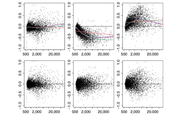
Relative signal versus signal intensity. Deviation plots, log(xi/v) versus log(v), much like the MA plots of Yang et al. [11] for the three replicate oligonucleotide arrays (from left to right) from HIV-infected samples. The top three plots show systematic deviations before normalization, and the bottom three show deviations after qspline normalization. Plots for prenormalized data show a comparison of curve fits for: log-intensity scaling (red); lowess (green); invariant set (magenta); and qspline normalizations (blue).
The signal-dependent biases for the individual channels of cDNA array data can be seen for an example glnA microarray in Figure 5 after print-tip scaling, lowess and qspline normalizations. In this case, log(G) and log(R) signals are compared to mean log(G) signals calculated over the six arrays. Although qspline normalized to signals calculated from all six arrays, normalization performance was comparable if not better than the lowess method that only used the Cy3 and Cy5 signals within each individual array. Additional examples can be found in the additional data files available with this paper (see Additional data files and [17]).
Figure 5.
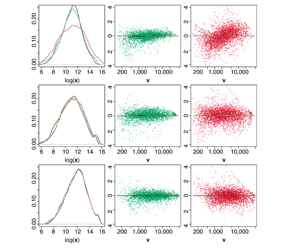
Relative signal versus signal intensity of cDNA array data. Signal distributions (left column) and MA plots (middle and right columns) for an example microarray after print-tip scaling (top row), scaled print-tip lowess (middle row) and scaled print-tip qspline (bottom row). Cy3 channels are shown in green, Cy5 channels in red and a running median curve is plotted in black.
Figure 6 compares lowess and qspline normalization to dye-swap normalization for replicate arrays A and B, where G A and R A were the control and mutant RNA samples on array A and G B and R B were the mutant and control samples on array B. Dye-swap normalization effectively averages log intensities within each sample type and is used to calculate a single set of log-ratios log((R A G B)/(G A R B)). From Figure 6 it is clear that dye-swap normalization alone is not enough to account for signal-dependent biases for this example. Either lowess or qspline alone provided more effective normalization than dye-swap averaging. This was due to the fact that, in this case, the dye bias was not consistent between replicates and can be seen to be much worse in array B. Signal-dependent normalization followed by dye-swap averaging should provide significantly better results than either approach alone.
Figure 6.
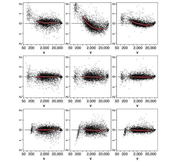
Effects of normalization on R/G ratios of dye-swapped arrays. MA plots for replicate arrays A and B showing log(R A/G A) (left column) log(R B/G B) (centre column) and dye-swap normalized log((R A G B)/(G A R B)) (right column). The top row shows standard dye-swap normalization of otherwise unnormalized data. The middle and bottom rows show scaled print-tip lowess and scaled print-tip qspline normalization of the individual arrays and the subsequent dye-swap averaging normalization.
When the signal-intensity range was separated into quartiles, the median log-ratio versus the probe means v was plotted for each array and each quartile. These medians can be seen in Figure 7 for the HIV, glnA and dye-swap experiments after the various normalizations. Separating these distributions by quartiles shows the performance of the normalization methods relative to signal intensity and again confirms the effectiveness of the methods described here. The lowess methods used for cDNA data were only employed to normalize within individual arrays and thus signal differences can still be observed between arrays. The R/G log-ratio variability for each array was found to be comparable for both single and multiple array normalization strategies. Again, the results from global and print-tip methods were not seen to differ.
Figure 7.
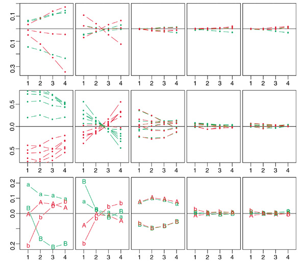
Median log-ratios by signal-based quartiles. Plots showing the median log-ratios (y axis) by quartiles (x axis) for each channel or array of experiments (rows) and for the different normalization methods (columns). The top row shows medians for the six arrays of the HIV experiment (control in green, HIV-infected in red) for data before normalization, after log-intensity scaling, lowess, rank-invariant set and qspline, respectively. The middle row shows medians for the 12 channels of the six glnA arrays (Cy3 in green and Cy5 in red) for data before normalization, log-intensity scaled by print-tip, scaled print-tip lowess, scaled print-tip qspline, and spatially scaled and smoothed (from left to right), respectively. The bottom row shows the four channels of the A. thaliana dye-swap replicate arrays 'A' and 'B', with wild-type channels in lower case, mutant in upper case, and with the same normalizations from left to right as were used in glnA plots above.
The distributions of R/G log-ratios versus print-tip can be compared for an example glnA array in Figure 8. After global normalization, a print-tip dependence can still be observed in most cases. Scaling the individual Cy3 and Cy5 log-signals before qspline normalization is shown to correct for some of this effect, although this method does not directly scale the R/G log-ratios. The scaled print-tip lowess first performs regressions by print-tip group, followed by tip-group scaling of the log-ratios and, not surprisingly, generates the most comparable print-tip log-ratio distributions. The preliminary spatial scaling technique also normalizes log-ratio information and can be seen to generate comparable print-tip log-ratio distributions.
Figure 8.
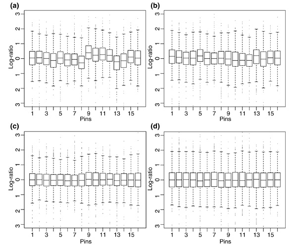
Box plots for R/G log-ratios by print tip. A strong print-tip bias can be seen after (a) global lowess or qspline but (b) is partially removed after scaling the R and G signals within each print-tip group before qspline normalization. Normalizing for (c) the spatial signal bias and (d) scaled print-tip lowess show more comparable tip distributions.
Spatial effects can be more or less dependent on the print-tip group, depending on the strength of the other spatial effects. Figure 9 shows an example from the dye-swap experiment where gradient effects tended to be as large as the print-tip effects. Tip-group normalization alone can be seen still to contain spatial bias within each tip sector. Spatial log-ratio normalization after global normalization can be seen to give the most homogeneous log-ratio signals across the surface of the array. An example oligonucleotide array is shown before and after spatial normalization, along with the values that were used for the normalization in Figure 10. The distribution of the log-signal differences used for the spatial normalization had a MAD of 0.014 for Affymetrix data compared to 0.3 for the cDNA array data of the glnA experiment, suggesting that spatial bias is more than ten times stronger for cDNA array data.
Figure 9.
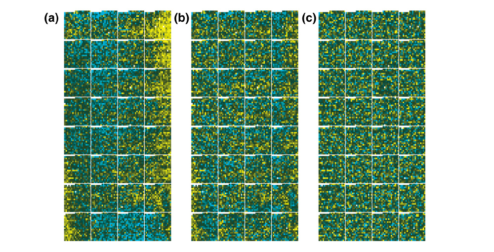
Spatial effects of normalization on R/G ratios. One of the two cDNA arrays from the dye-swap study showing Cy5/Cy3 log-ratios with a yellow-cyan color scale and indications defining the print-tip sectors. Upregulated probes are shown in yellow, unchanged in black and downregulated in cyan. (a) log-ratios after global qspline normalization where spatial and/or print-tip effects can clearly be seen. (b) The array after scaled print-tip lowess normalization; a noticeable improvement over the global approach is shown, but spatial bias within print-tip sectors can still be seen. (c) After spatial normalization little if any spatial bias can be seen.
Figure 10.
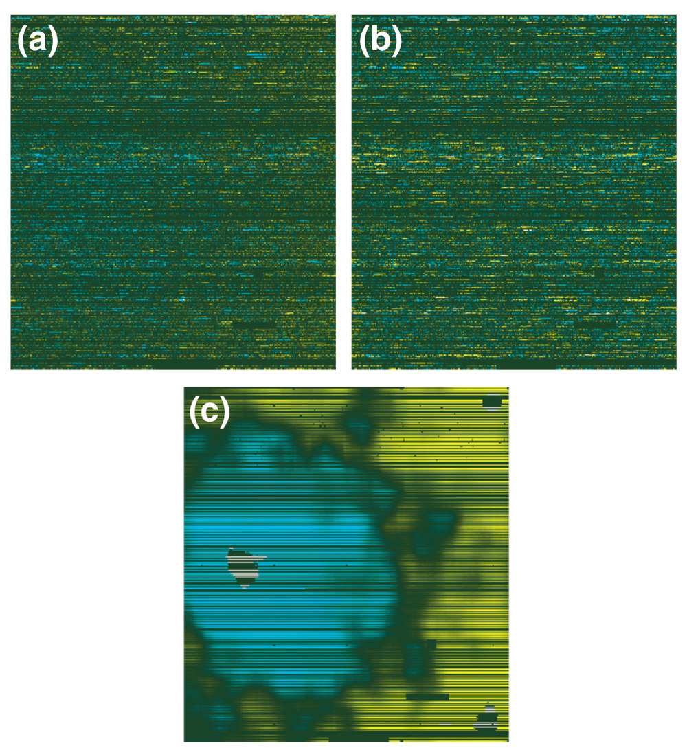
Spatial effects on oligonucleotide arrays. An example oligonucleotide array showing log-ratios of PM versus geometric mean PM in a yellow-cyan color scale. The omitted MM probes, shown in black, appear as horizontal stripes. (a) Relative PM values after global normalization; (b) results after spatial normalization. **(c)**The difference (of log(PM)) between the two, representing the spatial bias used for normalization.
Biological assessment of normalization
A set of genes was known to be differentially regulated in the glnA mutant strain of B. subtilis. These 41 genes were found to rank higher in a _t_-test analysis after signal-dependent normalization compared to rankings from unnormalized and scaled log-signals (Figure 11). A paired Welch _t-_test was performed on the individual Cy5 and Cy3 signals for each gene. The top 20 ranking genes can be seen in Figure 12, where the genes known to be differentially regulated are shown in parentheses and up- or downregulation is shown in red or green, respectively. Unnormalized data rankings showed only one of the 41 genes in the top 20 and overall these genes had an average rank corresponding to the 51st percentile, as would be expected from randomly selected genes. Log-signal scaling shifted the rankings of these genes to an average rank corresponding to the 20th percentile, whereas signal-dependent normalizations raised the average rank to correspond with the 8th to 9th percentile (2nd to 3rd percentile for the median rank). Seven of the 41 genes can be seen in the top 20 after scaled print-tip lowess and qspline. The spatial normalization approach appears to adversely effect the top 20 ranking genes though the resulting mean and median ranks of the 41 genes were comparable or better than the other approaches. The lowest average rank was observed for the global qspline method (8.1 percentile) followed closely by global and print-tip lowess both at the 8.5 percentile. The lowest median rank was seen for the spatial normalization results (1.9 percentile) followed by global qspline (2.4) and print-tip qspline (2.7).
Figure 11.
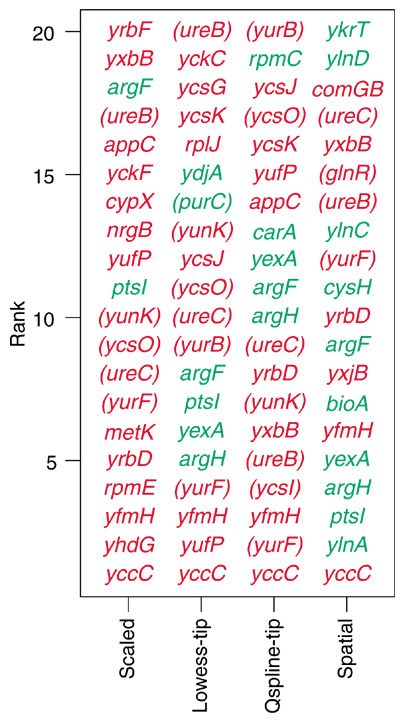
Top 20 _t_-test rankings for the glnA experiment. The B. subtilis genes found to be most significantly differentially regulated by the different normalization methods are shown. Genes known to be differentially regulated are in parenthesis. Genes in red are upregulated in the mutant strain whereas genes in green are downregulated.
Figure 12.
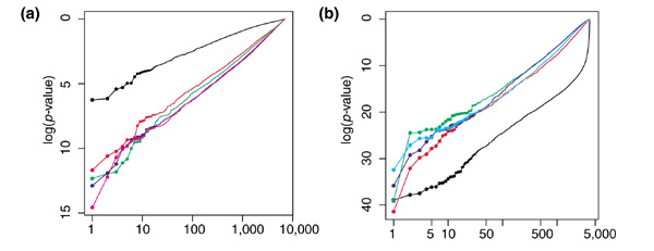
_t_-test rank versus log _p_-value. Log-log plots showing the distribution of _p_-values for (a) the HIV study and (b) the glnA study (right). p-values from unnormalized data (black) are compared to log-signal scaling (red), lowess (green), rank invariant (magenta), qspline (blue) and spatial normalization (cyan). Scaled print-tip lowess and qspline are shown for the cDNA data of the glnA experiment, whereas their global versions are shown for the oligonucleotide data.
_t_-tests were applied to gene-expression estimates calculated from the Li and Wong [1] reduced model for the oligonucleotide array data. Unfortunately, the set of genes believed to be differentially regulated due to HIV infection was found to be randomly distributed throughout the two sample _t_-test rankings both before and after different normalizations. The overall effects of normalization on the _p_-values can be seen for the HIV and glnA experiments in Figure 12. For this comparison, only the relative characteristics between normalization methods are of interest. The actual _p_-values are not correct as a result of multiple testing. Log rank versus log _p_-value plots show differing trends for oligonucleotide and cDNA array data. Unnormalized data show lower _p_-values for genes in the lower half of the ranking in cDNA because of the dye bias and lack of dye swapping over the six replicates, and suggest poorer signal-to-noise characteristics. Lack of normalization in the HIV experiment showed less significant _p_-values over all genes. Log-signal scaling showed slightly higher _p_-values whereas lowess, invariant set and qspline showed comparably lower _p_-values.
Discussion
Three important assumptions must hold for signal-dependent normalization methods. The first two were suggested by Zien et al. [18] in their linear centralization approach: the majority of genes are not differentially regulated (assumption 1); and the number of upregulated genes roughly equals the number downregulated (assumption 2). The third assumption is that these two assumptions hold across the signal-intensity range. Assumption 1 was used as a justification for centering log-ratio distributions and is likely to hold when an unbiased selection of thousands of genes is measured. If assumption 1 is true, then assumption 2 can be relaxed as long as random effects on non-differentially expressed genes are equally positive and negative. The third assumption is important for signal-dependent normalizations and is supported by the intuition that genes with 100 to 1,000 mRNA copies per cell will be no more or less biased toward up- or downregulation than genes with 10,000 to 100,000 copies per cell. Microarrays with a small number of genes may be biased to over- or underexpression and could generate data that do not conform to any of the listed assumptions. We believe that future microarrays will only include more features and genes, making these assumptions even more valid. In coming years, oligonucleotide arrays for humans will contain all 35,000 genes (or however many there may be) and therefore will not contain a biased selection of genes.
A potential fourth assumption motivates spatial- or pin-specific normalization and would state that assumption 2 should hold spatially across the surface of the array. These effects were observed to be more significant for cDNA microarrays, whereas global signal-dependent biases dominated over spatial effects for oligonucleotide array data. The MAD for the difference of log(PM) before and after global normalization was 30 times larger than the MAD of the difference between globally normalized and spatially normalized (0.3 versus 0.01). For the glnA experiment, the spatial effect as measured by a similar MAD was ten times larger than that of the HIV experiment but still roughly ten times smaller than the global cDNA effects (1.3 versus 0.1). Although spatial effects may not always be significant, probe-specific effects are a significant issue for oligonucleotide arrays, and must be addressed by other techniques such as the method of Li and Wong [2]. The preliminary spatial normalization method presented in this work will require further validation and development as the current method, by visual inspection, appears to be overfitting the cDNA data. Probe placement and microarray designs do not always correctly randomize strongly or weakly expressed genes, and may contain spatial biases that should not be removed. That said, the ranking of genes known to be regulated did not change significantly as a result of this overfitting.
The process of comparing and validating these methods should depend most heavily on the biological assessment. Unfortunately, this evidence was found to be the most unreliable. Genes from the list that were known to be differentially regulated were found throughout the _t_-test ranking in both the HIV and the glnA experiments. Statistical measures, such as reproducibility, were less ambiguous, but showed similar performance for global and print-tip, although clear print-tip biases were present. Each microarray system presented different sources of bias and in the end, no one criterion was sufficient for assessing whether microarray data was properly normalized. Observing global, signal-dependent and spatially dependent distributions is recommended in all cases.
Conclusions
Assessments of normalizations were shown globally for array signal and relative signal distributions as well as for signal-dependent MA-style plots and medians of relative signals by quartile. In all cases, these analyses showed favorable results for lowess, invariant set and qspline methods. Certain aspects of the spline-based methods make it preferable to the other methods. First, the qspline method is computationally more efficient than the lowess methods; second, owing to the random sampling procedure, lowess-based methods will give slightly different results for each data fitting whereas the spline methods are deterministic; and third, the quantile-based approach of qspline can normalize arrays with different numbers of features. Only through population-based methods, such as qspline, can arrays with different features be normalized for signal dependent bias.
Materials and methods
T-cell cultures infected with HIV
Ten million MT-4 cells were incubated with either 1 ml virus stock (2 multiplicity of infection (MOI) units of strain IIIB) or 1 ml mock virus for 3 h at 37°C. After extensive washing the cells were transferred to 80 cm3 Nunclon bottles in 20 ml culture medium (RPMI 1640 with 10% fetal calf serum and antibiotics) and cultured at 37°C, 5% CO2 for 7 days. Messenger RNA was extracted using QIAGEN RNeasy Mini kit and prepared for hybridization to Affymetrix HuGeneFL chips according to protocols provided by Affymetrix.
The Affymetrix HuGeneFL arrays contain about 1.4 × 10⁵ PM, MM probe pairs. Probe-based normalization was found to work on both PM and pooled PM, MM values, although the MM values were ignored in this analysis (We believe that MM values are unreliable indicators of cross-hybridization and can be shown to have a confounding effect on all but the top 20% of the signal intensity range.) Control features designed for grid alignment, spiked controls and ALU controls ("AFFX", "hum_alu") were removed.
Bacillus cultures on cDNA microarrays
Cells were grown at 37°C in a modified Spizizen salt-buffered minimal medium as described previously [19] supplemented with 100 μg/ml L-tryptophan. Na2SO4 was used instead of (NH4)2SO4 and glutamine (0.2%) was added as the sole nitrogen source. At an OD = 1 (450 nm), approximately 100 ml of culture was harvested by centrifugation at 7,000 rpm for 5 min. The pellet was resuspended in 400 μl water and RNA was isolated from this by the use of four tubes from the fastRNA kit blue (BIO 101, Carlsbad, CA) and as recommended by the supplier. cDNA synthesis, dye coupling of probe, array, hybridization and scanning were carried out as described by DeRisi and co-workers (protocol available at [20]). RNA preparations were run in duplicate and each sample was hybridized to triplicate arrays. In all cases the control RNA was labeled with Cy5 and treatment RNA with Cy3. Each of the 4,100 genes was spotted on the array twice, which gave 12 measurements per gene per experiment.
Microarray normalization
The variance within replicate group was estimated for each normalization described below,

where i is an index over n probe signals, and j is an index over m replicates.
Global scaling of log intensities
As a comparison with the signal-dependent qspline and lowess approaches, a scaling of log intensities was carried out as follows. Probe intensities were log-transformed (in all cases, we used log base 2 on signal-intensity data) and a measure of central tendency, c j, was calculated for each array and for the entire matrix (c). The mean of the log values was used but the median was found to work just as well. Each array was then scaled in the log-space to the global mean, log(xj)(c/c j). This simple transformation often accounted for much of the variability between oligonucleotide arrays. The approach used on cDNA array data scaled each Cy3 and Cy5 channel to the same central tendency with the additional constraint that each print-tip group also had the same Cy3 and Cy5 central tendency.
Lowess normalizations
The Affymetrix normalization method found in the Raffy module of the sma package uses the lowess function ('loess') with a robust local linear regression mode ('symmetric'). The Raffy method performed all pairwise normalizations between the six HIV arrays and averaged the five results (_m_-1) for each array. The process was then repeated on the new data, which resulted in 30 total fits for the six arrays. Instead of averaging all pairwise array regressions on a single random sample of feature pairs, the modified version averaged iterative regressions between each array and the target array using a new random sample on each iteration. This resulted in 18 total fits for the six arrays. The former method tended to undernormalize and did not perform as well as simple log-intensity scaling. The adapted method used essentially the same procedure and code but performed significantly better when used in this scheme.
The six replicates for each glnA and tnrA experiment were normalized to a prototype, v, denned by the median or geometric mean of the six Cy3 channels used to measure the control mRNA (wild type). By this method, all 12 channels from the six arrays were normalized to each other and at the same time the Cy5 channels were normalized to the Cy3 channels. The cDNA normalization method found in the Rarray module of the sma package uses the lowess function ('lowess') with analogous settings as described for oligonucleotide array normalization. Both global and scaled print-tip group lowess normalization were performed (norm = 'l' and norm = 's', respectively). The scaled print-tip mode performed lowess normalization for within each print-tip group and then scaled the log-ratios of each group by its respective MAD [11].
Cubic spline normalization using quantiles
For this approach, all signal channels are normalized to a target array. The same method was used for cDNA and oligonucleotide array data.
The geometric mean of each probe was calculated over all arrays, xj, in the experiment,

where j indexed over the m = 6 arrays and i indexed over the n probes.
From each array and the vector v, 100 quantiles were taken, qj andqv (percentiles). The size of the quantile sample represented < 0.1% of n. Figure 1 shows an example comparison of array signal distributions xj and v along with a quantile-quantile plot showing the correlation between the corresponding qj and qv. Each qv,qj pair was used to fit a cubic spline function, s j = f(qv,qj), where f was a spline function generator that fits the parameters of a natural cubic spline (B-spline). The splinefun function in the R base package was used for this purpose. Spline parameters were fit for each interval between consecutive quantiles. The interpolating spline function defined over the _k_th interval, is defined for the parameters ajk and y jk in Equation 3. For an unsmoothed cubic spline, y jk = q vk,
s j(x) = a _jk_1 + a _jk_2 (_x_-y jk) + a _jk_3 (_x_-y jk)2 + a _jk_4 (_x_-y jk)3 (3)
In an iterative approach, quantiles were resampled from percentiles shifted by a small offset _np_0/k where _p_0 was the first percentile and k the number of iterations (defines the difference in rank between consecutive quantiles). This provided a different set of evenly spaced quantiles for each curve fitting. For the normalizations performed here, the results from five interpolations were averaged. The qspline method was implemented in R and included in the Bioconductor package, which will be described elsewhere and is available from the web [21].
Data for cDNA experiments were qspline normalized with percentile samples and fitted in an iterative approach as described for the oligonucleotide arrays. The signal distributions were found to contain many non-smooth features not common for both channels. To account for the print-tip effect, an additional normalization was performed where Cy3 and Cy5 signals were scaled within each print-tip group, as described in global scaling of log intensities, before qspline normalization as just described.
Spatial normalization
Local signal (log-ratio) was estimated for each probe using a weighted mean of neighboring probe signals. A sliding square window centered on the each probe (50 × 50 for oligonucleotide arrays, and 10 × 10 for cDNA) was used to define the local neighborhood. Weights were defined by their Euclidean distance to the center probe using a Gaussian function (standard deviation 19 for 50 × 50 neighborhood and 3 for the 10 × 10 neighborhood). For both oligonucleotide and cDNA array data, this adjustment was made after global qspline normalization.
Additional data files
Additional data files showing MA plots and signal distributions from all the HIV, glnA, tnrA arrays for the different normalizations are available with the online version of this paper and at [17].
Supplementary Material
Additional data file 1
MA plots and signal distributions from all the HIV arrays
Additional data file 2
MA plots and signal distributions from all the glnA arrays
Additional data file 3
MA plots and signal distributions from all the tnrA arrays
Acknowledgments
Acknowledgements
C.W., S.B. and S.K. acknowledge the Danish National Research Foundation for financial support. L.G. was supported by a grant from the Danish Biotechnology Instrument Center. H.J. would like to thank Maria Tang and Alan Sloma at Novozymes Biotechnology, Davis.
References
- Li C, Wong WH. Model-based analysis of oligonucleotide arrays: Expression index computation and outlier detection. Proc Natl Acad Sci USA. 2001;98:31–36. doi: 10.1073/pnas.011404098. [DOI] [PMC free article] [PubMed] [Google Scholar]
- Li C, Wong WH. Model-based analysis of oligonucleotide arrays: model validation, design issues and standard error application. Genome Biol. 2001;2:research0032.1–0032.11. doi: 10.1186/gb-2001-2-8-research0032. [DOI] [PMC free article] [PubMed] [Google Scholar]
- Schadt EE, Li C, Su C, Wong WH. Analyzing high-density oligonucleotide gene expression array data. J Cell Biochem. 2000;80:192–202. [PubMed] [Google Scholar]
- Schadt EE, Li C, Ellis B, Wong WH. Feature extraction and normalization algorithms for high-density oligonucleotide gene expression array data. J Cell Biochem. 2001;Suppl 37:120–125. doi: 10.1002/jcb.10073. [DOI] [PubMed] [Google Scholar]
- Cavalieri D, Townsend JP, Hartl DL. Manifold anomalies in gene expression in a vineyard isolate of Saccharomyces cerevisiae revealed by DNA microarray analysis. Proc Natl Acad Sci USA. 2000;97:12369–12374. doi: 10.1073/pnas.210395297. [DOI] [PMC free article] [PubMed] [Google Scholar]
- Golub TR, Slonim DK, Tamayo P, Huard C, Gaasenbeek M, Mesirov JP, Coller H, Loh ML, Downing JR, Caligiuri MA, et al. Molecular classification of cancer: class discovery and class prediction by gene expression monitoring. Science. 1999;286:531–537. doi: 10.1126/science.286.5439.531. [DOI] [PubMed] [Google Scholar]
- Virtaneva K, Wright FA, Tanner SM, Yuan B, Lemon WJ, Caligiuri MA, Bloomfield CD, de la Chapelle A, Krahe R. Expression profiling reveals fundamental biological differences in acute myeloid leukemia with isolated trisomy 8 and normal cytogenetics. Proc Natl Acad Sci USA. 2001;98:1124–1129. doi: 10.1073/pnas.98.3.1124. [DOI] [PMC free article] [PubMed] [Google Scholar]
- Kerr K, Martin M, Churchill G. Analysis of variance for gene expression microarray data. J Comput Biol. 2000;7:819–837. doi: 10.1089/10665270050514954. [DOI] [PubMed] [Google Scholar]
- Zolotukhin I, Lange J. Application of analysis of variance schemes to expression data. In Proceedings of the German Conference on Bioinformatics Berlin: Logos Verlag; 2000. pp. 159–166.
- Pollack JR, Perou CM, Alizadeh AA, Eisen MB, Pergamenschikov A, Williams CF, Jeffrey SS, Botstein D, Brown PO. Genome-wide analysis of DNA copy-number changes using cDNA microarrays. Nat Genet. 1999;23:41–46. doi: 10.1038/12640. [DOI] [PubMed] [Google Scholar]
- Yang YH, Dudoit S, Luu P, Lin DM, Peng V, Ngai J, Speed TP. Normalization for cDNA microarray data: a robust composite method addressing single and multiple slide systematic variation. Nucleic Acids Res. 2002;30:e15. doi: 10.1093/nar/30.4.e15. [DOI] [PMC free article] [PubMed] [Google Scholar]
- Chiang DY, Brown PO, Eisen MB. Visualizing associations between genome sequences and gene expression data using genome-mean expression profiles. Bioinformatics. 2001;17:S49–S55. doi: 10.1093/bioinformatics/17.suppl_1.s49. [DOI] [PubMed] [Google Scholar]
- Tseng GC, Oh MK, Rohlin L, Liao JC, Wong WH. Issues in cDNA microarray analysis: quality filtering, channel normalization, models of variations and assessment of gene effects. Nucleic Acids Res. 2001;29:2549–2557. doi: 10.1093/nar/29.12.2549. [DOI] [PMC free article] [PubMed] [Google Scholar]
- Cleveland WS, Grosse E, Shyu WM. Local regression models. In: Chambers JM, Hastie TJ, editor. In Statistical Models in S. Pacific Grove, CA: Wadsworth & Brooks/Cole;; 1992. p. Chapter 8. [Google Scholar]
- The Comprehensive R Archive Network http://cran.us.r-project.org
- R package: statistics for microarray analysis http://www.stat.berkeley.edu/users/terry/zarray/Software/smacode.html
- Additional figures http://www.cbs.dtu.dk/~workman/qspline
- Zien A, Aigner T, Zimmer R, Lengauer T. Centralization: a new method for the normalization of gene expression data. Bioinformatics. 2001;17:s323–s331. doi: 10.1093/bioinformatics/17.suppl_1.s323. [DOI] [PubMed] [Google Scholar]
- Saxild HH, Jacobsen JH, Nygaard P. Functional analysis of the Bacillus subtilis purT gene encoding formate-dependent glycinamide ribonucleotide transformylase. Microbiology. 1995;141:2211–2218. doi: 10.1099/13500872-141-9-2211. [DOI] [PubMed] [Google Scholar]
- Microarrays.org http://www.microarrays.org
- BioConductor: software for bioinformatics http://www.bioconductor.org
Associated Data
This section collects any data citations, data availability statements, or supplementary materials included in this article.
Supplementary Materials
Additional data file 1
MA plots and signal distributions from all the HIV arrays
Additional data file 2
MA plots and signal distributions from all the glnA arrays
Additional data file 3
MA plots and signal distributions from all the tnrA arrays